Capital Budgeting Techniques for Feasibility Analysis

This document discusses capital budgeting techniques like discounted cash flow methods to determine project feasibility. It explains the importance of net present value (NPV) and discount rate in decision making. The document also provides calculations and analysis for Kidman Resources' WACC and NPV for two alternative scenarios.

REPORT

EXECUTIVE SUMMARY
Capital budgeting techniques like discounted cash flow methods can be used to determine the
feasibility of projects such as choosing between building a new refinery or outsourcing the
process.
There are various methods that can be used in capital budgeting. The most common method is
the net present value (NPV). A positive NPV suggests that the project is feasible, whereas a
negative NPV suggests a project is not feasible.
One of the key assumptions required in calculating the NPV is the discount rate. Care must be
taken when choosing a discount rate as a low rate may result in the company choosing projects
that are otherwise not feasible. The same applies in the reverse.
1

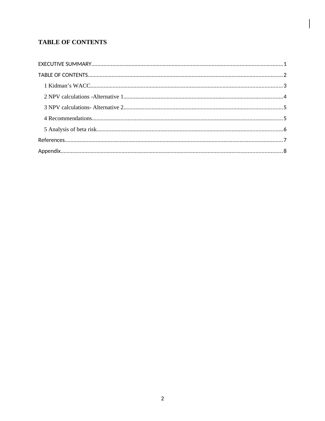
TABLE OF CONTENTS
EXECUTIVE SUMMARY.................................................................................................................................1
TABLE OF CONTENTS...................................................................................................................................2
1 Kidman’s WACC.................................................................................................................................3
2 NPV calculations -Alternative 1...........................................................................................................4
3 NPV calculations- Alternative 2...........................................................................................................5
4 Recommendations................................................................................................................................5
5 Analysis of beta risk.............................................................................................................................6
References...................................................................................................................................................7
Appendix.....................................................................................................................................................8
2

1 Kidman’s WACC
Step 1: Cost of Equity
Cost of Equity = Rf + Beta*(Rm –Rf), where Rf is the risk free rate and Rm is the return on the
market (Investing Answers, 2019).
It has been given that the risk-free rate is 2.28 % p.a., and the return on the market is 7.70 % p.a.
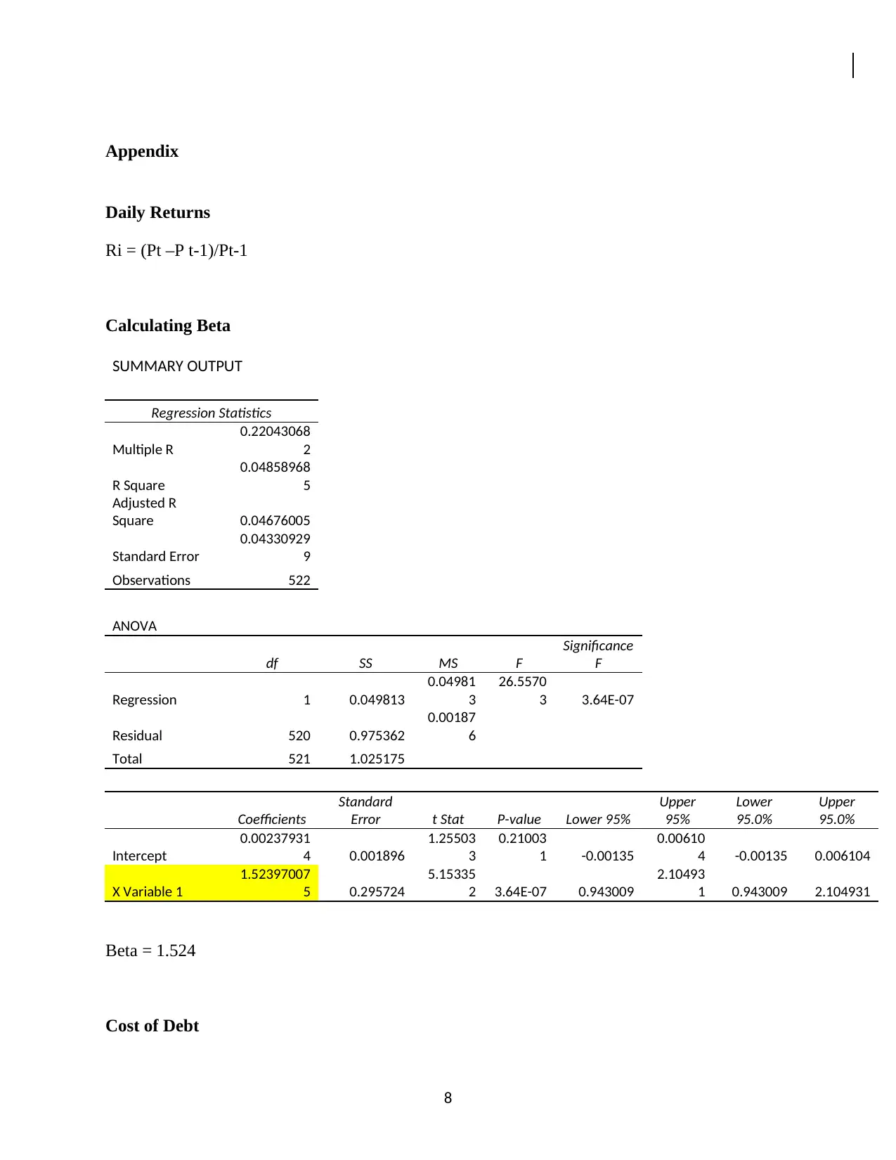
By regressing Kidman’s daily return and the market index, a beta value of 1.52 is obtained.
Hence, using the CAPM model, Kidman Resources cost of equity is given as 10.54%
Step 2: Cost of Debt
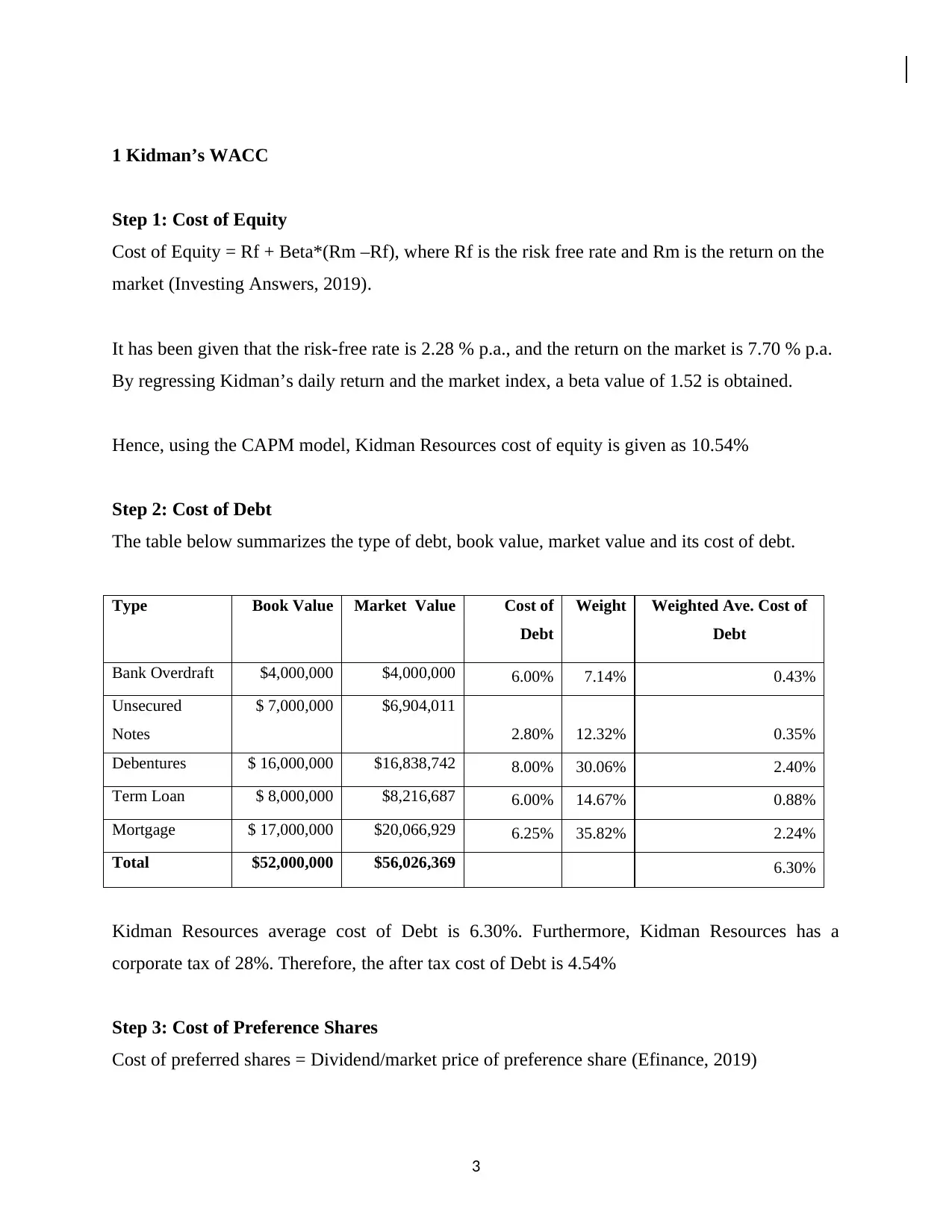
The table below summarizes the type of debt, book value, market value and its cost of debt.
Type Book Value Market Value Cost of
Debt
Weight Weighted Ave. Cost of
Debt
Bank Overdraft $4,000,000 $4,000,000 6.00% 7.14% 0.43%
Unsecured
Notes
$ 7,000,000 $6,904,011
2.80% 12.32% 0.35%
Debentures $ 16,000,000 $16,838,742 8.00% 30.06% 2.40%
Term Loan $ 8,000,000 $8,216,687 6.00% 14.67% 0.88%
Mortgage $ 17,000,000 $20,066,929 6.25% 35.82% 2.24%
Total $52,000,000 $56,026,369 6.30%
Kidman Resources average cost of Debt is 6.30%. Furthermore, Kidman Resources has a
corporate tax of 28%. Therefore, the after tax cost of Debt is 4.54%
Step 3: Cost of Preference Shares
Cost of preferred shares = Dividend/market price of preference share (Efinance, 2019)
3

Currently, Kidman Resources holds 1,500,000 preference shares (par value $ 1 per share) with
5% dividends selling for $0.60 per share. Hence, Kidman Resources cost of preferred shares is
8.33%.
Step 4: Weighted Average Cost of Capital
WACC =Weight Debt * cost of debt *(1 – T) + Weight equity *cost of equity+ Weight
Preference shares *cost of Preference shares (CFI, 2019)
Where T is the corporate tax
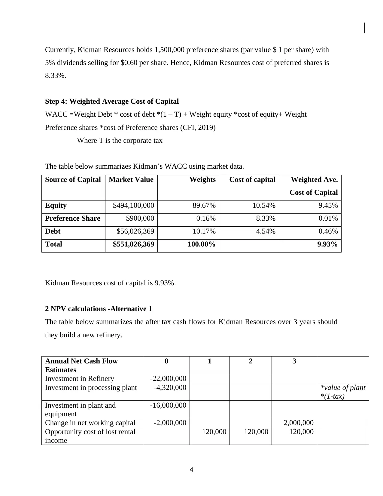
The table below summarizes Kidman’s WACC using market data.
Source of Capital Market Value Weights Cost of capital Weighted Ave.
Cost of Capital
Equity $494,100,000 89.67% 10.54% 9.45%
Preference Share $900,000 0.16% 8.33% 0.01%
Debt $56,026,369 10.17% 4.54% 0.46%
Total $551,026,369 100.00% 9.93%
Kidman Resources cost of capital is 9.93%.
2 NPV calculations -Alternative 1
The table below summarizes the after tax cash flows for Kidman Resources over 3 years should
they build a new refinery.
Annual Net Cash Flow
Estimates
0 1 2 3
Investment in Refinery -22,000,000
Investment in processing plant -4,320,000 *value of plant
*(1-tax)
Investment in plant and
equipment
-16,000,000
Change in net working capital -2,000,000 2,000,000
Opportunity cost of lost rental
income
120,000 120,000 120,000
4

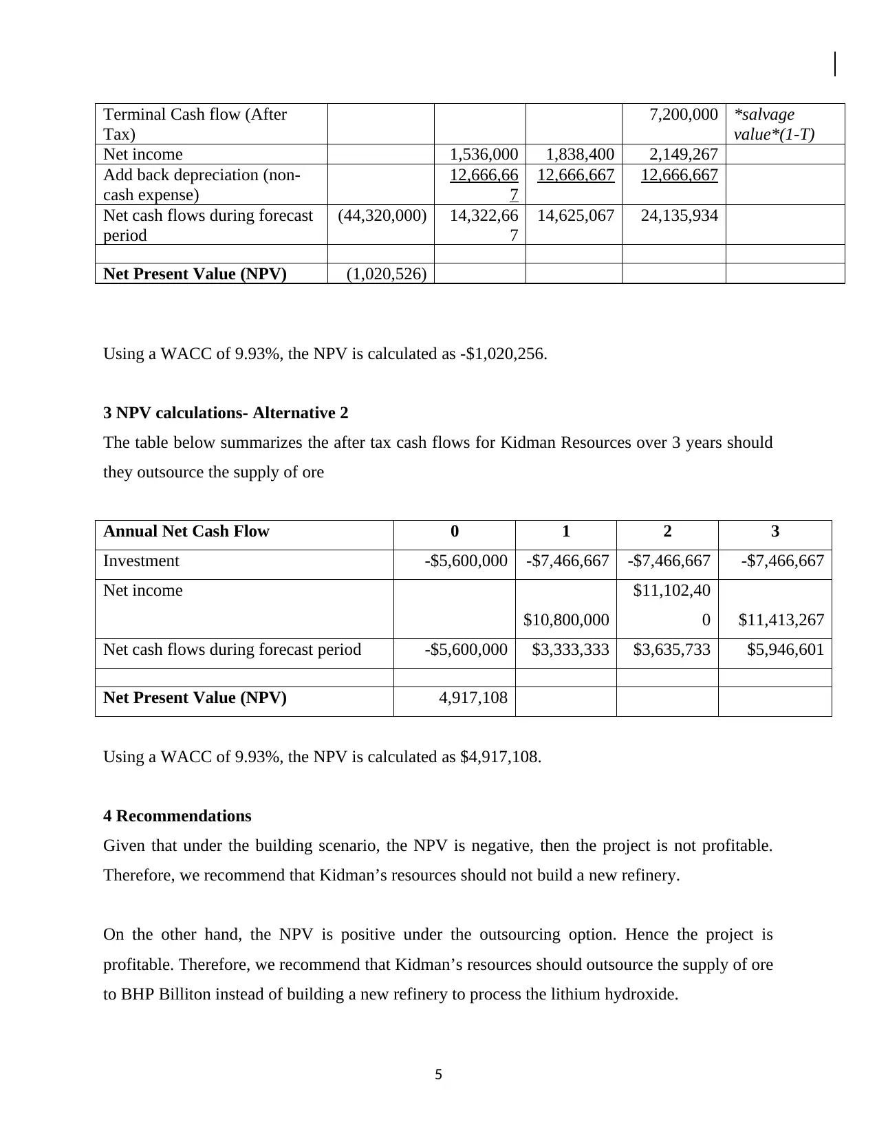
Terminal Cash flow (After
Tax)
7,200,000 *salvage
value*(1-T)
Net income 1,536,000 1,838,400 2,149,267
Add back depreciation (non-
cash expense)
12,666,66
7
12,666,667 12,666,667
Net cash flows during forecast
period
(44,320,000) 14,322,66
7
14,625,067 24,135,934
Net Present Value (NPV) (1,020,526)
Using a WACC of 9.93%, the NPV is calculated as -$1,020,256.
3 NPV calculations- Alternative 2
The table below summarizes the after tax cash flows for Kidman Resources over 3 years should
they outsource the supply of ore
Annual Net Cash Flow 0 1 2 3
Investment -$5,600,000 -$7,466,667 -$7,466,667 -$7,466,667
Net income
$10,800,000
$11,102,40
0 $11,413,267
Net cash flows during forecast period -$5,600,000 $3,333,333 $3,635,733 $5,946,601
Net Present Value (NPV) 4,917,108
Using a WACC of 9.93%, the NPV is calculated as $4,917,108.
4 Recommendations
Given that under the building scenario, the NPV is negative, then the project is not profitable.
Therefore, we recommend that Kidman’s resources should not build a new refinery.
On the other hand, the NPV is positive under the outsourcing option. Hence the project is
profitable. Therefore, we recommend that Kidman’s resources should outsource the supply of ore
to BHP Billiton instead of building a new refinery to process the lithium hydroxide.
5

5 Analysis of beta risk
Beta measures the volatility of an individual stock portfolio in comparison to the unsystematic
risk of the entire market (Investopedia, 2019). Examples of risks and events that may cause
Kidman’s resources beta to significantly change include:
 Businesses change over the year and are exposed to different economic cycles.
 The length of the interval used in the calculation of Beta -analyst prefer 5 year intervals,
anything too short or longer may lead to errors in estimation.
 Beta is only valid as the data used to calculate it. For example, the market index used in
the regression may not capture the systematic risk completely (Goetzmann, 2018).
Increase in Beta
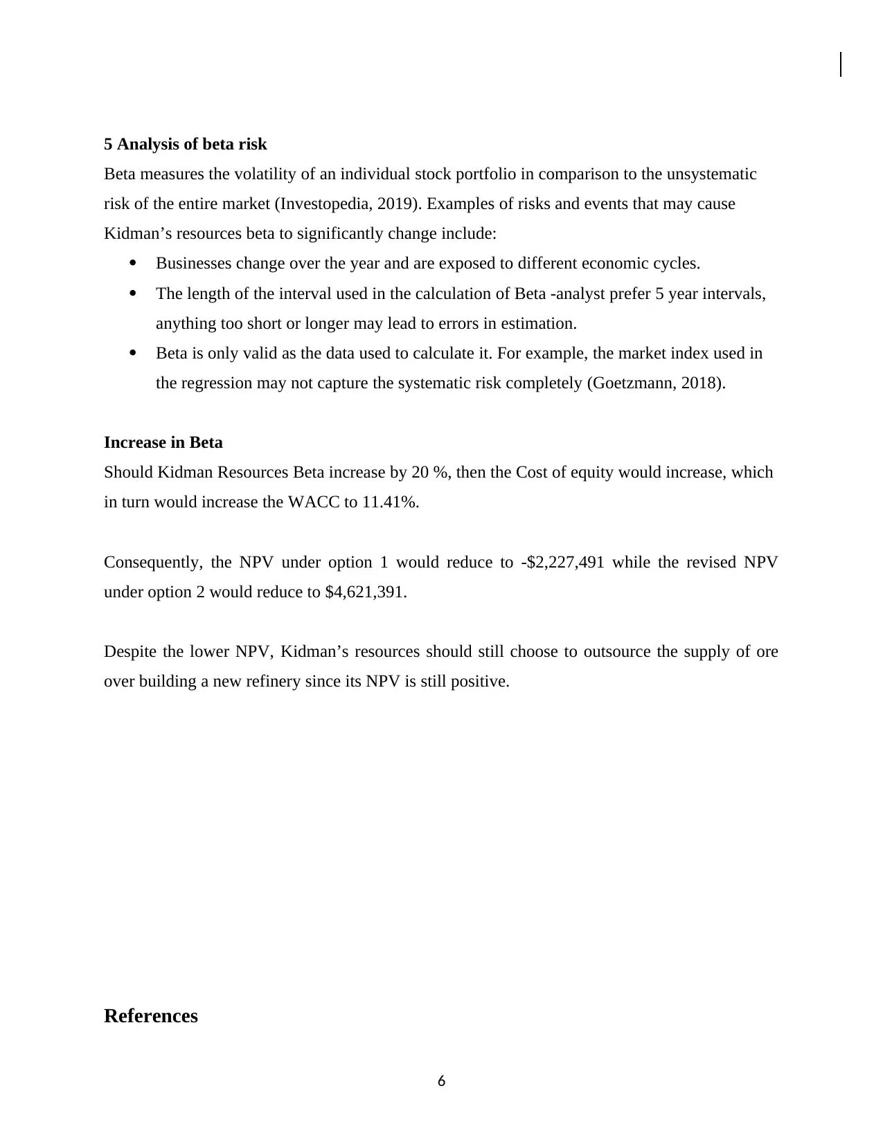
Should Kidman Resources Beta increase by 20 %, then the Cost of equity would increase, which
in turn would increase the WACC to 11.41%.
Consequently, the NPV under option 1 would reduce to -$2,227,491 while the revised NPV
under option 2 would reduce to $4,621,391.
Despite the lower NPV, Kidman’s resources should still choose to outsource the supply of ore
over building a new refinery since its NPV is still positive.
References
6

Accounting Explained. (2017). Capital Budgeting. Retrieved September 2017, from Accounting
Explained: http://accountingexplained.com/managerial/capital-budgeting/
CFI. (2019). Definition of WACC. Retrieved from
https://corporatefinanceinstitute.com/resources/knowledge/finance/what-is-wacc-formula/
Efinance. (2019). Cost of Preference Share Capital. Retrieved from
https://efinancemanagement.com/investment-decisions/cost-of-preference-share-capital
Goetzmann, W. (2018). An Introduction to Investment Theory. YALE School of Management.
Investing Answers. (2019). Gordon Growth Model. Retrieved from
https://investinganswers.com/financial-dictionary/income-dividends/gordon-growth-model-
5270
Investopedia. (2019). What Beta Means When Considering a Stock's Risk. Retrieved from
https://www.investopedia.com/investing/beta-know-risk/
Tucker, J. (2009). How to set the hurdle rate for capital investments. Retrieved from
https://www.eprints.uwe.ac.uk/11334/1/Tucker_2009_QFinance_book_chapter.doc
7

Appendix
Daily Returns
Ri = (Pt –P t-1)/Pt-1
Calculating Beta
SUMMARY OUTPUT
Regression Statistics
Multiple R
0.22043068
2
R Square
0.04858968
5
Adjusted R
Square 0.04676005
Standard Error
0.04330929
9
Observations 522
ANOVA
df SS MS F
Significance
F
Regression 1 0.049813
0.04981
3
26.5570
3 3.64E-07
Residual 520 0.975362
0.00187
6
Total 521 1.025175
Coefficients
Standard
Error t Stat P-value Lower 95%
Upper
95%
Lower
95.0%
Upper
95.0%
Intercept
0.00237931
4 0.001896
1.25503
3
0.21003
1 -0.00135
0.00610
4 -0.00135 0.006104
X Variable 1
1.52397007
5 0.295724
5.15335
2 3.64E-07 0.943009
2.10493
1 0.943009 2.104931
Beta = 1.524
Cost of Debt
8

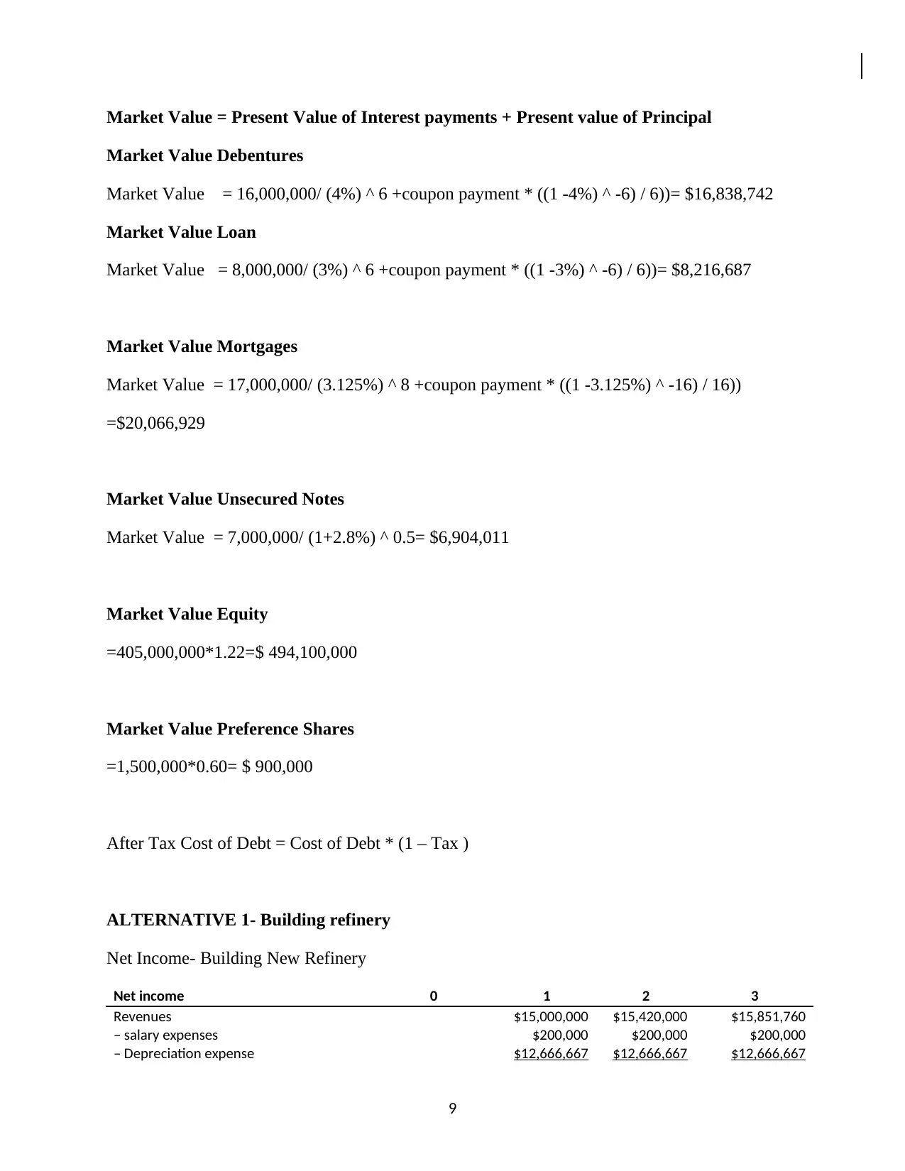
Market Value = Present Value of Interest payments + Present value of Principal
Market Value Debentures
Market Value = 16,000,000/ (4%) ^ 6 +coupon payment * ((1 -4%) ^ -6) / 6))= $16,838,742
Market Value Loan
Market Value = 8,000,000/ (3%) ^ 6 +coupon payment * ((1 -3%) ^ -6) / 6))= $8,216,687
Market Value Mortgages
Market Value = 17,000,000/ (3.125%) ^ 8 +coupon payment * ((1 -3.125%) ^ -16) / 16))
=$20,066,929
Market Value Unsecured Notes
Market Value = 7,000,000/ (1+2.8%) ^ 0.5= $6,904,011
Market Value Equity
=405,000,000*1.22=$ 494,100,000
Market Value Preference Shares
=1,500,000*0.60= $ 900,000
After Tax Cost of Debt = Cost of Debt * (1 – Tax )
ALTERNATIVE 1- Building refinery
Net Income- Building New Refinery
Net income 0 1 2 3
Revenues $15,000,000 $15,420,000 $15,851,760
– salary expenses $200,000 $200,000 $200,000
– Depreciation expense $12,666,667 $12,666,667 $12,666,667
9

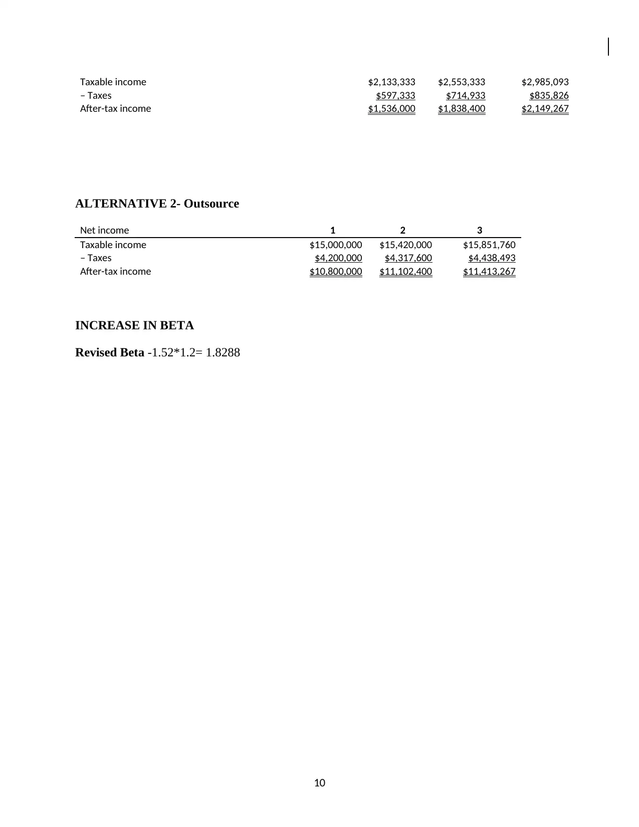
Taxable income $2,133,333 $2,553,333 $2,985,093
– Taxes $597,333 $714,933 $835,826
After-tax income $1,536,000 $1,838,400 $2,149,267
ALTERNATIVE 2- Outsource
Net income 1 2 3
Taxable income $15,000,000 $15,420,000 $15,851,760
– Taxes $4,200,000 $4,317,600 $4,438,493
After-tax income $10,800,000 $11,102,400 $11,413,267
INCREASE IN BETA
Revised Beta -1.52*1.2= 1.8288
10