Financial Modeling and Analysis of Boeing Stock

This assignment delves into the financial modeling and analysis of Boeing stock. It employs a capital asset pricing model (CAPM) to assess the relationship between market returns and Boeing's excess return. The analysis includes calculating the beta coefficient, performing regression analysis to determine the sensitivity of Boeing's stock to market movements, testing for normality of error terms, and evaluating the neutrality of the stock using a 95% confidence interval.

Statistics
Name
University
6th October 2017

Table of Contents
Introduction......................................................................................................................................3
Methodology....................................................................................................................................3
Descriptive statistics........................................................................................................................4
Summary statistics.......................................................................................................................4
Time series plots..........................................................................................................................4
Hypothesis Test...............................................................................................................................7
Testing whether the average return on Boeing stock is at least 3%.............................................7
Comparison of risk associated with stocks..................................................................................8
Comparison of average returns....................................................................................................9
Estimating the CAPM using linear regression...........................................................................10
Confidence interval to test neutrality of stock...........................................................................11
Testing normality of error term..................................................................................................12
References......................................................................................................................................14

Introduction
This report presents analysis of four different stocks. The main aim is to give a comparison of the
stocks in terms of volatility and risk. The research question we sought to answer is which of the
four stock would one choose? Data was downloaded from Yahoo Finance where the start time
was 01/12/2010 and the end time was 31/05/2016 (a total of 65 months were included for
analysis). The sample portion of the data is shown in table 1 below;
Table 1: Sample portion of the data
Closing stock Stock Returns
Date
S&P 500
index
IBM
Stock
Price
US TN
(10 year)
Boeing
Stock Price
S&P
500
index
IBM
Stock
Price
US TN
(10 year)
Boeing
Stock Price
12/1/201
0
1257.64
0 146.760 3.305 65.260
1/1/2011
1286.12
0 162.000 3.378 69.480 2.239 9.880 2.185 6.266
2/1/2011
1327.22
0 161.880 3.414 72.010 3.146 -0.074 1.060 3.577
3/1/2011
1325.83
0 163.070 3.454 73.930 -0.105 0.732 1.165 2.631
4/1/2011
1363.61
0 170.580 3.296 79.780 2.810 4.502 -4.682 7.615
5/1/2011
1345.20
0 168.930 3.050 78.030 -1.359 -0.972 -7.757 -2.218
6/1/2011
1320.64
0 171.550 3.158 73.930 -1.843 1.539 3.480 -5.397
7/1/2011
1292.28
0 181.850 2.805 70.470 -2.171 5.831 -11.854 -4.793
8/1/2011
1218.89
0 171.910 2.218 66.860 -5.847 -5.621 -23.480 -5.259
9/1/2011
1131.42
0 174.870 1.924 60.510 -7.447 1.707 -14.220 -9.979
10/1/201
1
1253.30
0 184.630 2.175 65.790 10.231 5.431 12.262 8.366
Methodology
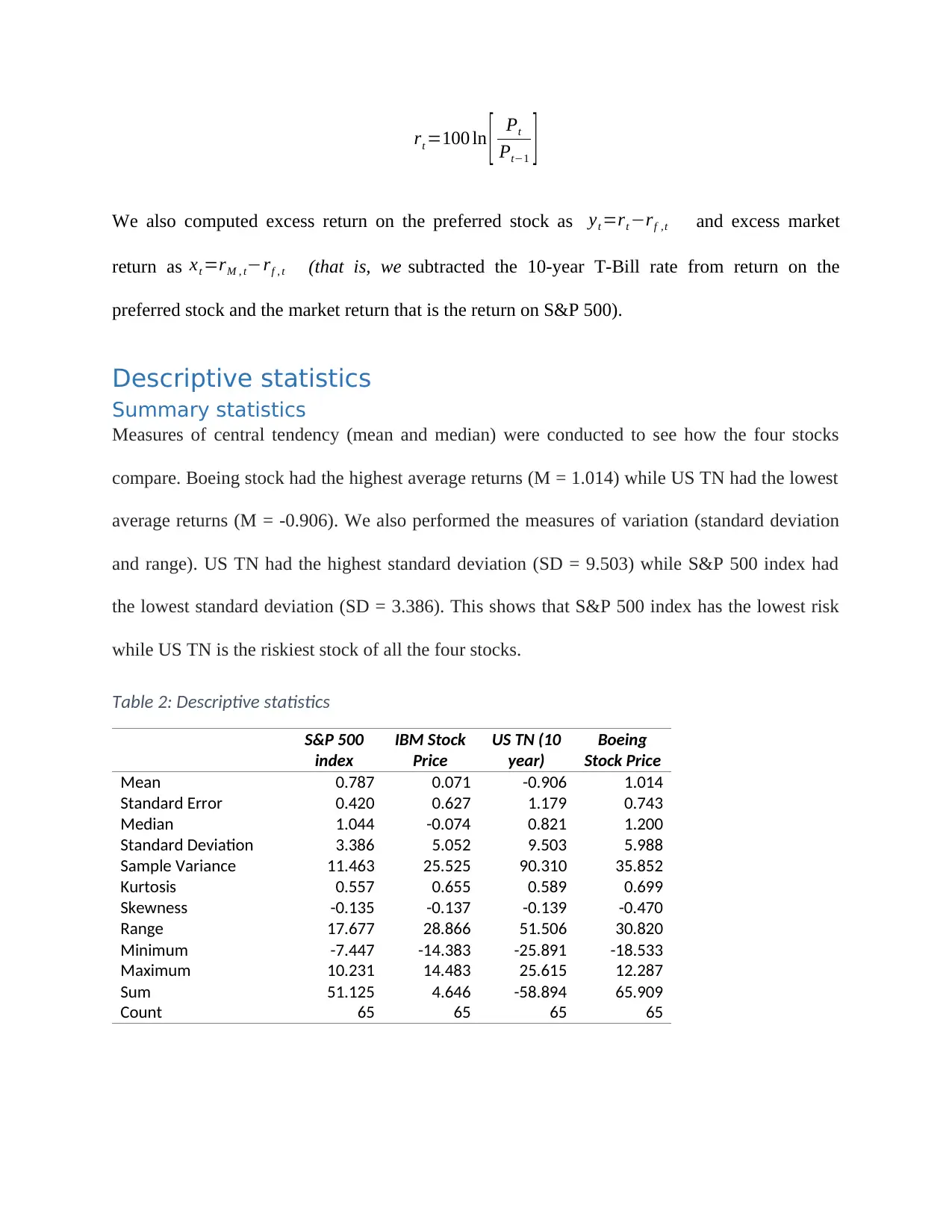
Data was presented in excel and then transformed for purposes of conducting analysis on it.
Excel was used for analysis where the data analysis add in was heavily utilized. The stock
returns was computed using the following formula;

rt =100 ln [ Pt
Pt−1 ]
We also computed excess return on the preferred stock as yt =rt −rf ,t and excess market
return as xt =rM , t−rf , t (that is, we subtracted the 10-year T-Bill rate from return on the
preferred stock and the market return that is the return on S&P 500).
Descriptive statistics
Summary statistics
Measures of central tendency (mean and median) were conducted to see how the four stocks
compare. Boeing stock had the highest average returns (M = 1.014) while US TN had the lowest
average returns (M = -0.906). We also performed the measures of variation (standard deviation
and range). US TN had the highest standard deviation (SD = 9.503) while S&P 500 index had
the lowest standard deviation (SD = 3.386). This shows that S&P 500 index has the lowest risk
while US TN is the riskiest stock of all the four stocks.
Table 2: Descriptive statistics
S&P 500
index
IBM Stock
Price
US TN (10
year)
Boeing
Stock Price
Mean 0.787 0.071 -0.906 1.014
Standard Error 0.420 0.627 1.179 0.743
Median 1.044 -0.074 0.821 1.200
Standard Deviation 3.386 5.052 9.503 5.988
Sample Variance 11.463 25.525 90.310 35.852
Kurtosis 0.557 0.655 0.589 0.699
Skewness -0.135 -0.137 -0.139 -0.470
Range 17.677 28.866 51.506 30.820
Minimum -7.447 -14.383 -25.891 -18.533
Maximum 10.231 14.483 25.615 12.287
Sum 51.125 4.646 -58.894 65.909
Count 65 65 65 65

Time series plots
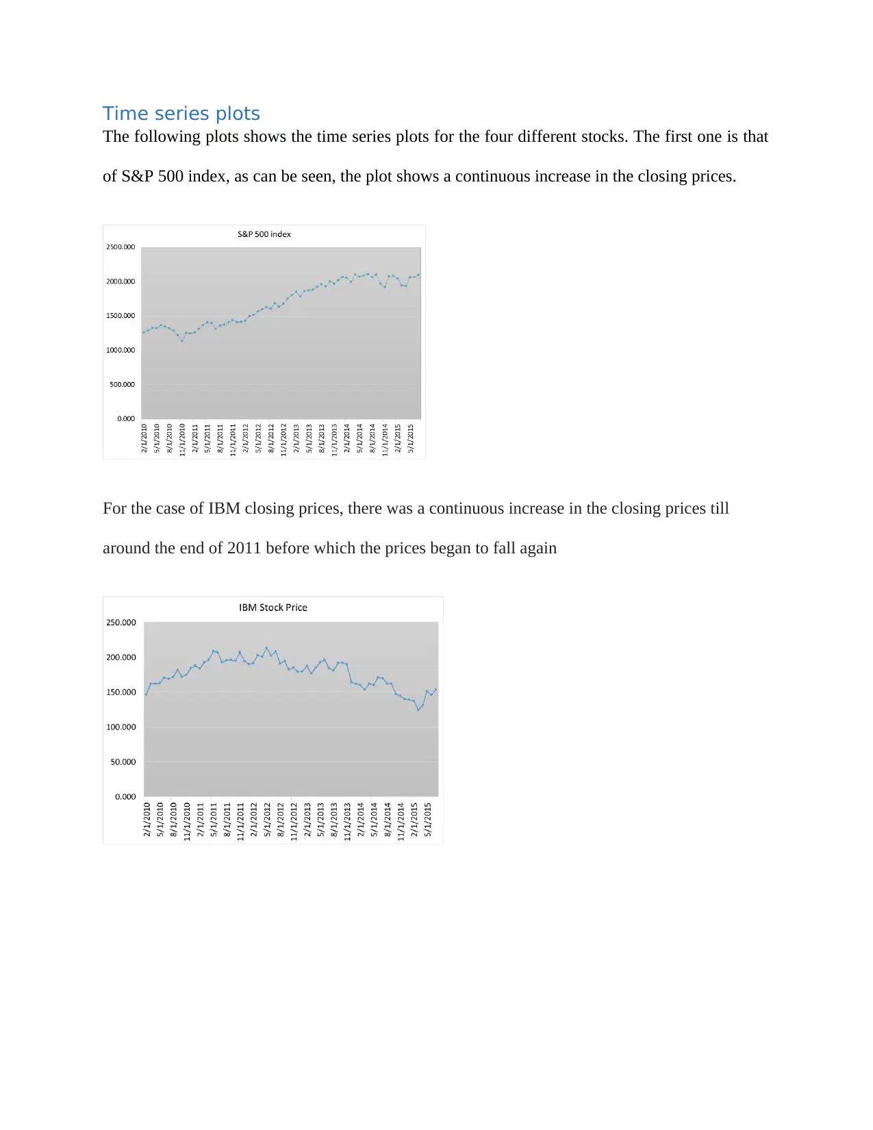
The following plots shows the time series plots for the four different stocks. The first one is that
of S&P 500 index, as can be seen, the plot shows a continuous increase in the closing prices.
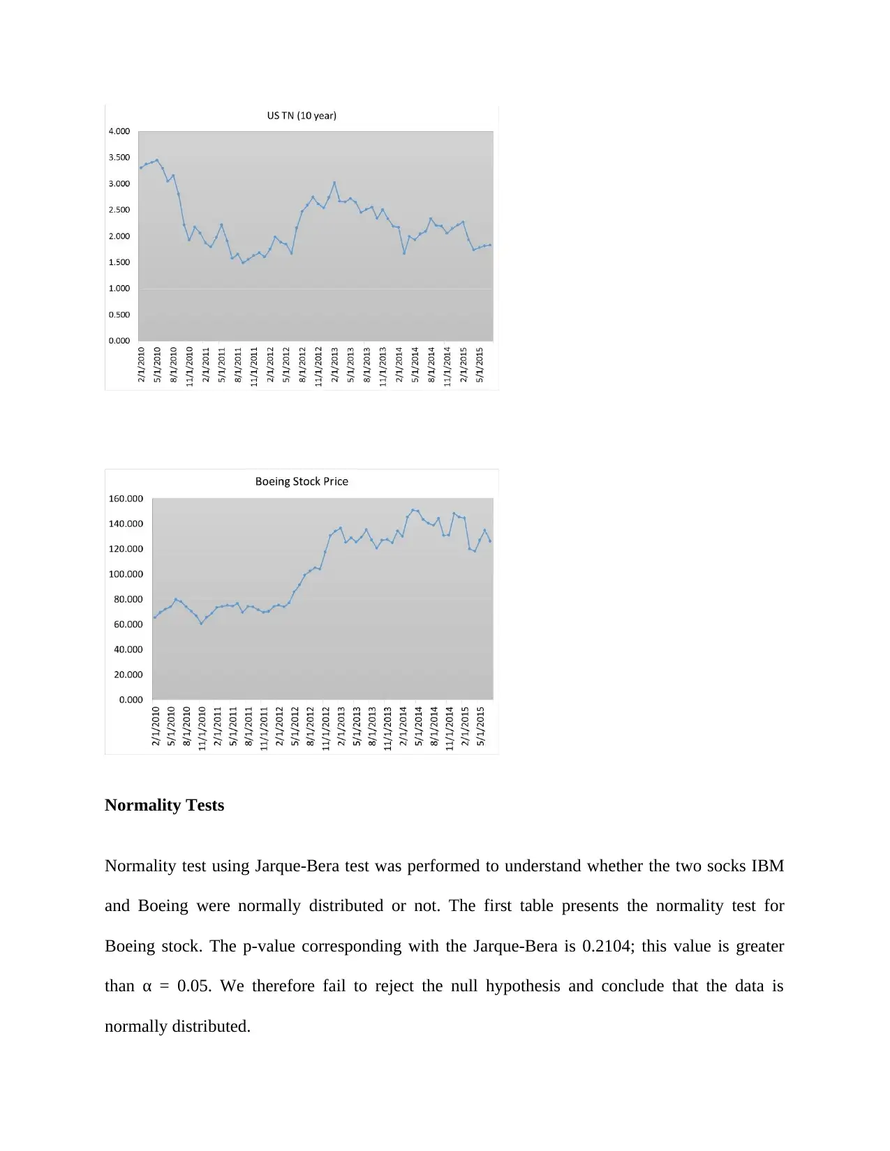
For the case of IBM closing prices, there was a continuous increase in the closing prices till
around the end of 2011 before which the prices began to fall again

Normality Tests
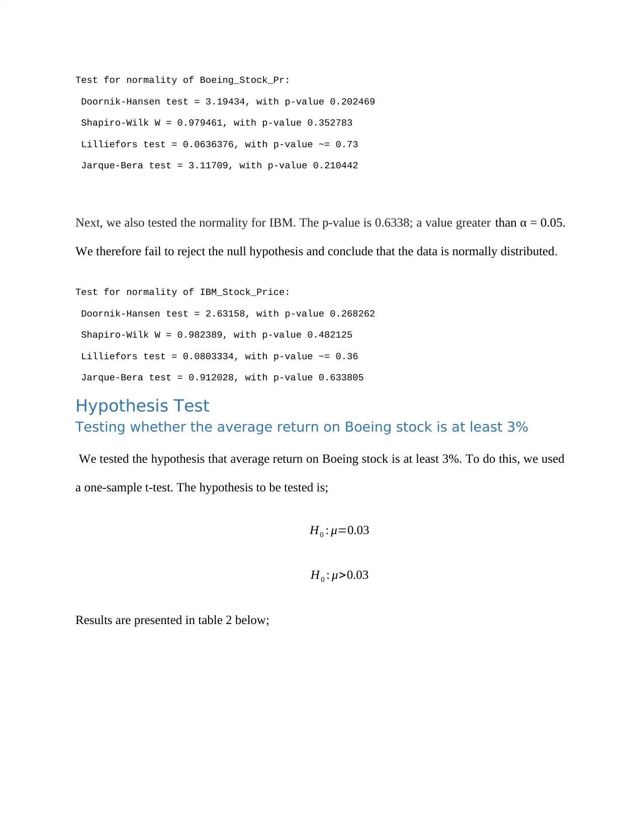
Normality test using Jarque-Bera test was performed to understand whether the two socks IBM
and Boeing were normally distributed or not. The first table presents the normality test for
Boeing stock. The p-value corresponding with the Jarque-Bera is 0.2104; this value is greater
than α = 0.05. We therefore fail to reject the null hypothesis and conclude that the data is
normally distributed.

Test for normality of Boeing_Stock_Pr:
Doornik-Hansen test = 3.19434, with p-value 0.202469
Shapiro-Wilk W = 0.979461, with p-value 0.352783
Lilliefors test = 0.0636376, with p-value ~= 0.73
Jarque-Bera test = 3.11709, with p-value 0.210442
Next, we also tested the normality for IBM. The p-value is 0.6338; a value greater than α = 0.05.
We therefore fail to reject the null hypothesis and conclude that the data is normally distributed.
Test for normality of IBM_Stock_Price:
Doornik-Hansen test = 2.63158, with p-value 0.268262
Shapiro-Wilk W = 0.982389, with p-value 0.482125
Lilliefors test = 0.0803334, with p-value ~= 0.36
Jarque-Bera test = 0.912028, with p-value 0.633805
Hypothesis Test
Testing whether the average return on Boeing stock is at least 3%
We tested the hypothesis that average return on Boeing stock is at least 3%. To do this, we used
a one-sample t-test. The hypothesis to be tested is;
H0 : μ=0.03
H0 : μ>0.03
Results are presented in table 2 below;

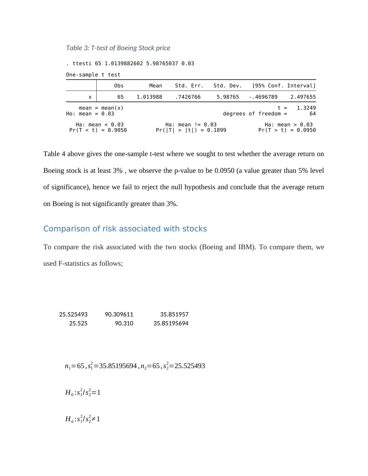
Table 3: T-test of Boeing Stock price
Pr(T < t) = 0.9050 Pr(|T| > |t|) = 0.1899 Pr(T > t) = 0.0950
Ha: mean < 0.03 Ha: mean != 0.03 Ha: mean > 0.03
Ho: mean = 0.03 degrees of freedom = 64
mean = mean(x) t = 1.3249
x 65 1.013988 .7426766 5.98765 -.4696789 2.497655
Obs Mean Std. Err. Std. Dev. [95% Conf. Interval]
One-sample t test
. ttesti 65 1.0139882602 5.98765037 0.03
Table 4 above gives the one-sample t-test where we sought to test whether the average return on
Boeing stock is at least 3% , we observe the p-value to be 0.0950 (a value greater than 5% level
of significance), hence we fail to reject the null hypothesis and conclude that the average return
on Boeing is not significantly greater than 3%.
Comparison of risk associated with stocks
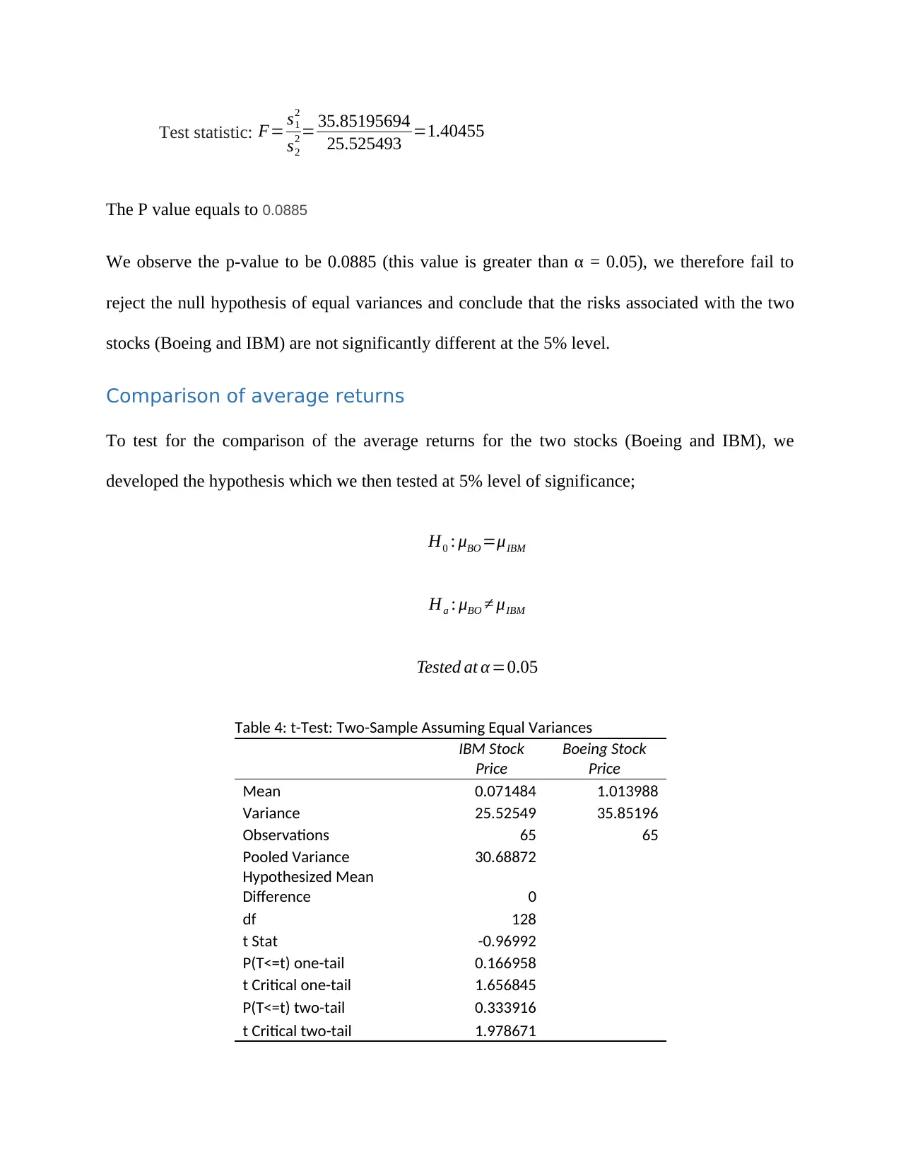
To compare the risk associated with the two stocks (Boeing and IBM). To compare them, we
used F-statistics as follows;
25.525493 90.309611 35.851957
25.525 90.310 35.85195694
n1=65 , s1
2 =35.85195694 , n2=65 , s2
2=25.525493
H0 :s1
2 /s2
2=1
Ha :s1
2 /s2
2 ≠ 1

Test statistic: F= s1
2
s2
2 = 35.85195694
25.525493 =1.40455
The P value equals to 0.0885
We observe the p-value to be 0.0885 (this value is greater than α = 0.05), we therefore fail to
reject the null hypothesis of equal variances and conclude that the risks associated with the two
stocks (Boeing and IBM) are not significantly different at the 5% level.
Comparison of average returns
To test for the comparison of the average returns for the two stocks (Boeing and IBM), we
developed the hypothesis which we then tested at 5% level of significance;
H0 : μBO =μIBM
Ha : μBO ≠ μIBM
Tested at α=0.05
Table 4: t-Test: Two-Sample Assuming Equal Variances
IBM Stock
Price
Boeing Stock
Price
Mean 0.071484 1.013988
Variance 25.52549 35.85196
Observations 65 65
Pooled Variance 30.68872
Hypothesized Mean
Difference 0
df 128
t Stat -0.96992
P(T<=t) one-tail 0.166958
t Critical one-tail 1.656845
P(T<=t) two-tail 0.333916
t Critical two-tail 1.978671

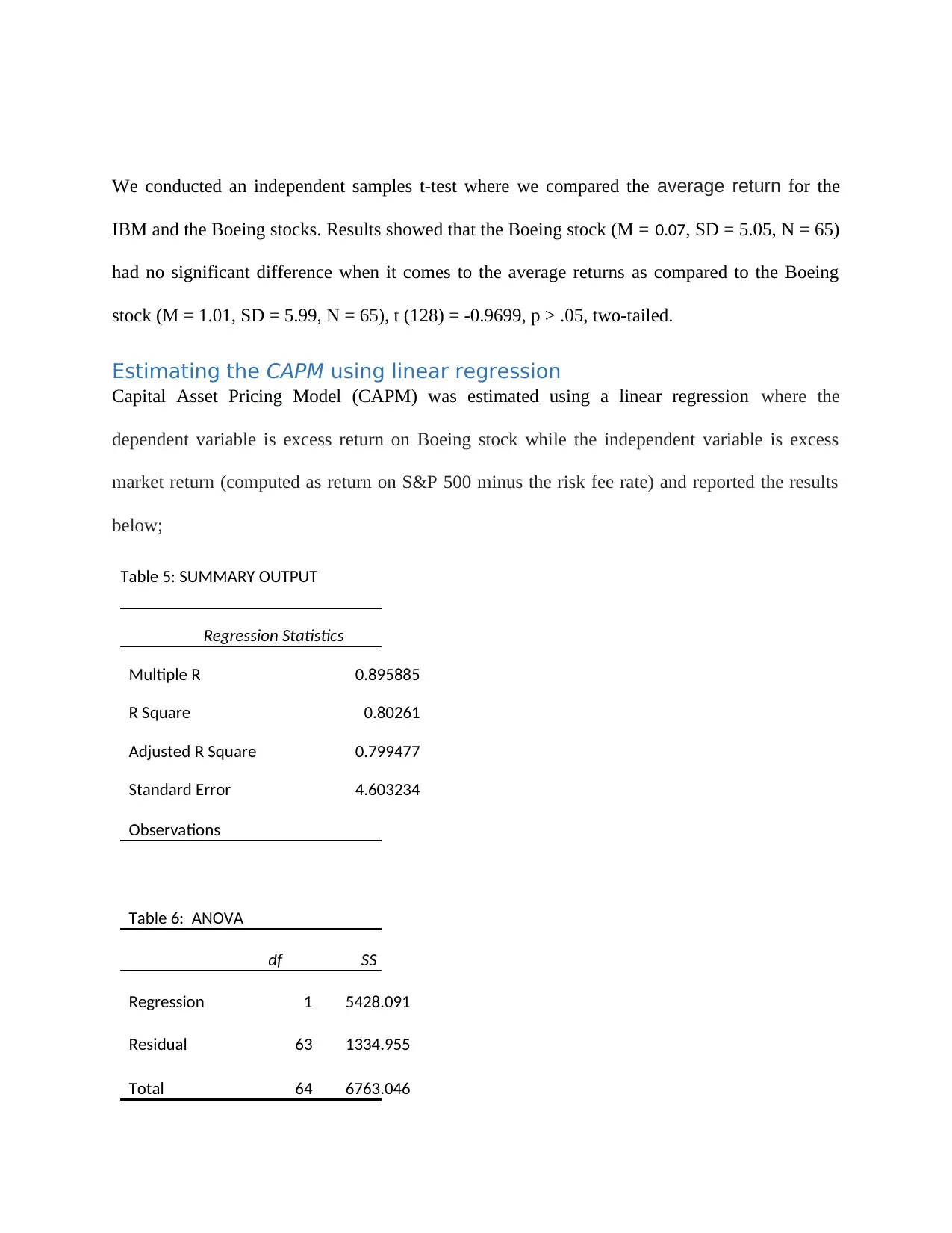
We conducted an independent samples t-test where we compared the average return for the
IBM and the Boeing stocks. Results showed that the Boeing stock (M = 0.07, SD = 5.05, N = 65)
had no significant difference when it comes to the average returns as compared to the Boeing
stock (M = 1.01, SD = 5.99, N = 65), t (128) = -0.9699, p > .05, two-tailed.
Estimating the CAPM using linear regression
Capital Asset Pricing Model (CAPM) was estimated using a linear regression where the
dependent variable is excess return on Boeing stock while the independent variable is excess
market return (computed as return on S&P 500 minus the risk fee rate) and reported the results
below;
Table 5: SUMMARY OUTPUT
Regression Statistics
Multiple R 0.895885
R Square 0.80261
Adjusted R Square 0.799477
Standard Error 4.603234
Observations
Table 6: ANOVA
df SS
Regression 1 5428.091
Residual 63 1334.955
Total 64 6763.046

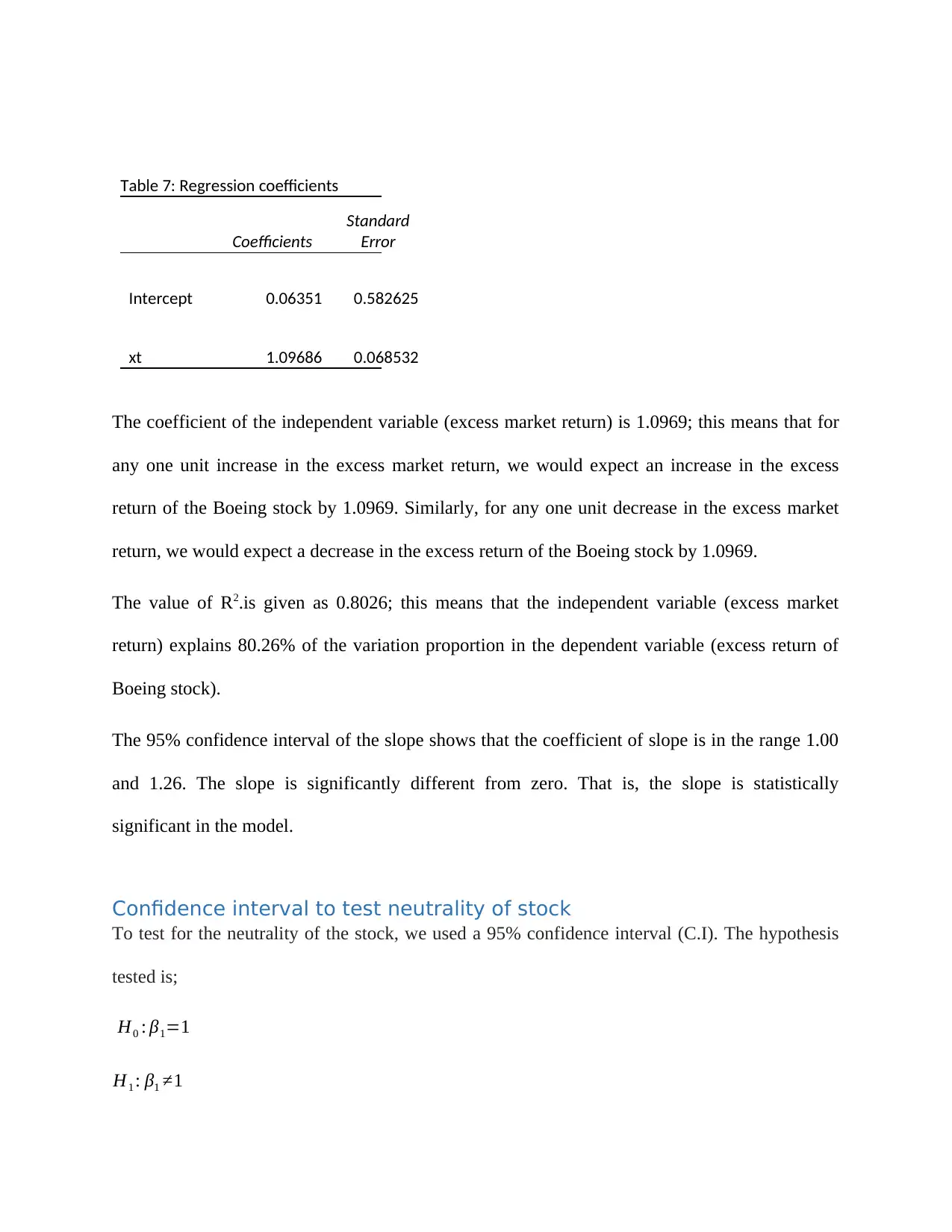
Table 7: Regression coefficients
Coefficients
Standard
Error
Intercept 0.06351 0.582625
xt 1.09686 0.068532
The coefficient of the independent variable (excess market return) is 1.0969; this means that for
any one unit increase in the excess market return, we would expect an increase in the excess
return of the Boeing stock by 1.0969. Similarly, for any one unit decrease in the excess market
return, we would expect a decrease in the excess return of the Boeing stock by 1.0969.
The value of R2.is given as 0.8026; this means that the independent variable (excess market
return) explains 80.26% of the variation proportion in the dependent variable (excess return of
Boeing stock).
The 95% confidence interval of the slope shows that the coefficient of slope is in the range 1.00
and 1.26. The slope is significantly different from zero. That is, the slope is statistically
significant in the model.
Confidence interval to test neutrality of stock
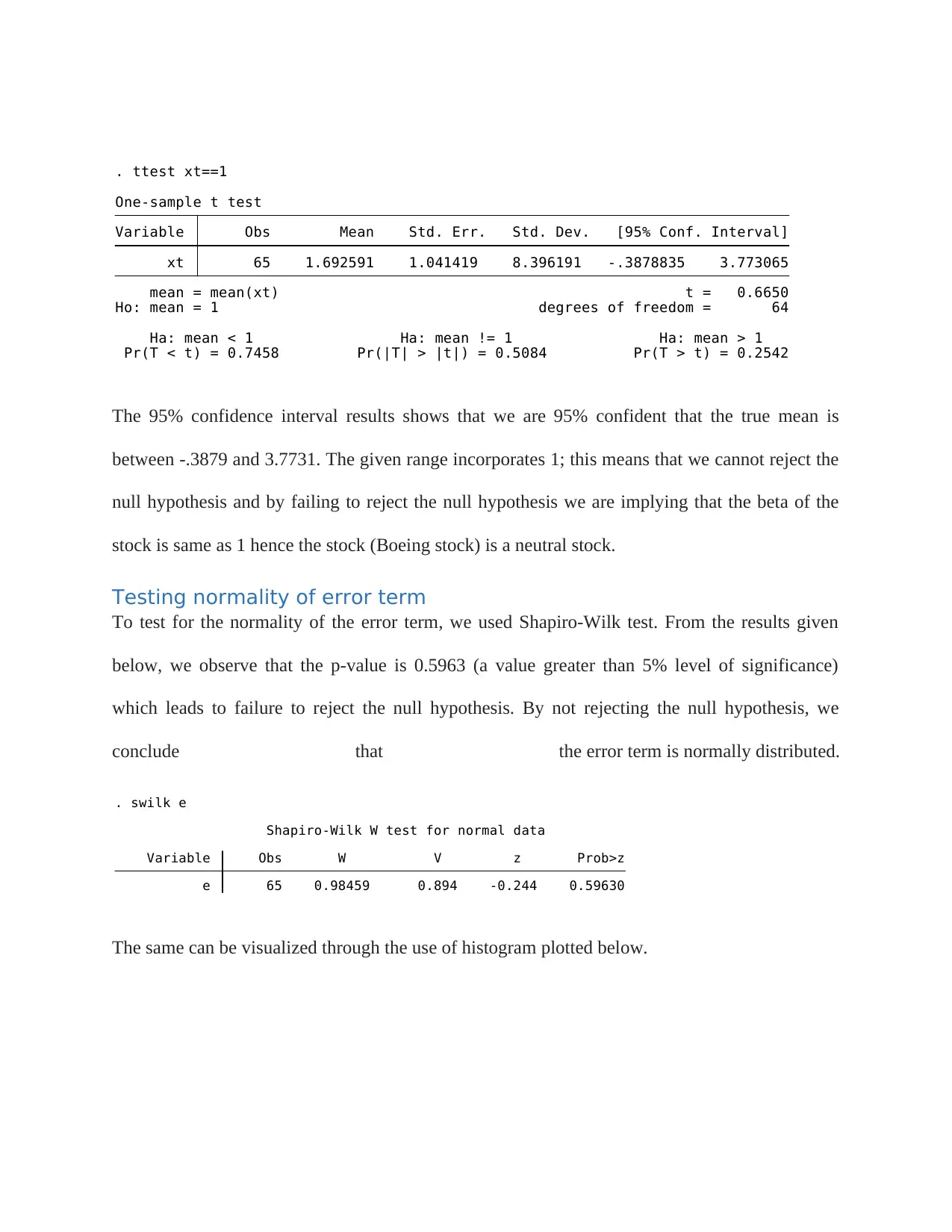
To test for the neutrality of the stock, we used a 95% confidence interval (C.I). The hypothesis
tested is;
H0 : β1=1
H1 : β1 ≠1

Pr(T < t) = 0.7458 Pr(|T| > |t|) = 0.5084 Pr(T > t) = 0.2542
Ha: mean < 1 Ha: mean != 1 Ha: mean > 1
Ho: mean = 1 degrees of freedom = 64
mean = mean(xt) t = 0.6650
xt 65 1.692591 1.041419 8.396191 -.3878835 3.773065
Variable Obs Mean Std. Err. Std. Dev. [95% Conf. Interval]
One-sample t test
. ttest xt==1
The 95% confidence interval results shows that we are 95% confident that the true mean is
between -.3879 and 3.7731. The given range incorporates 1; this means that we cannot reject the
null hypothesis and by failing to reject the null hypothesis we are implying that the beta of the
stock is same as 1 hence the stock (Boeing stock) is a neutral stock.
Testing normality of error term
To test for the normality of the error term, we used Shapiro-Wilk test. From the results given
below, we observe that the p-value is 0.5963 (a value greater than 5% level of significance)
which leads to failure to reject the null hypothesis. By not rejecting the null hypothesis, we
conclude that the error term is normally distributed.
e 65 0.98459 0.894 -0.244 0.59630
Variable Obs W V z Prob>z
Shapiro-Wilk W test for normal data
. swilk e
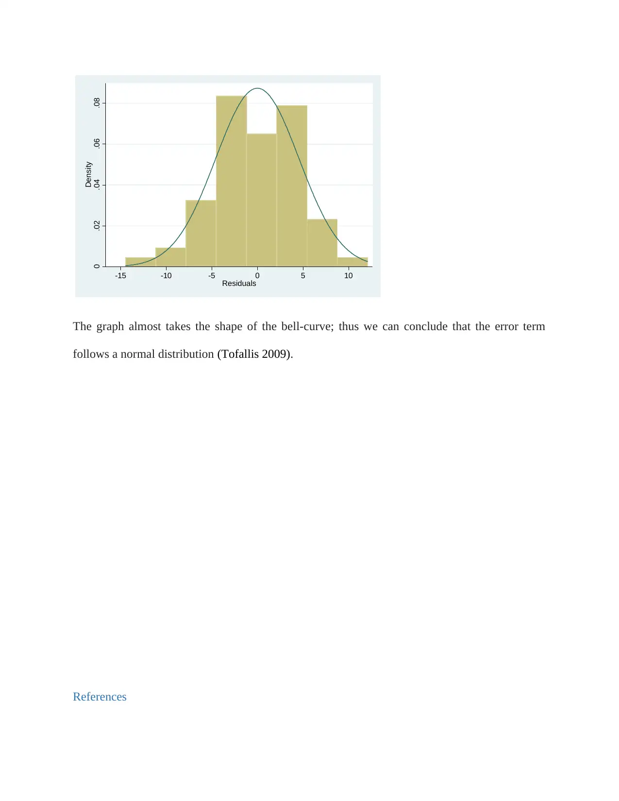
The same can be visualized through the use of histogram plotted below.

0 .02 .04 .06 .08
Density
-15 -10 -5 0 5 10
Residuals
The graph almost takes the shape of the bell-curve; thus we can conclude that the error term
follows a normal distribution (Tofallis 2009).
References