Research Methodology

This document provides an overview of research methodology and its applications in regression analysis, logistic regression, and ANOVA. It discusses the assumptions and variables involved in each method. The document also includes model summaries, coefficient tables, and explanations of statistical significance. References are provided for further reading.

Running head: Research Methodology 1
Research Methodology
By:
Student ID:
Course No:
Tutor:
Date:

Research Methodology 2
Question 1
a)
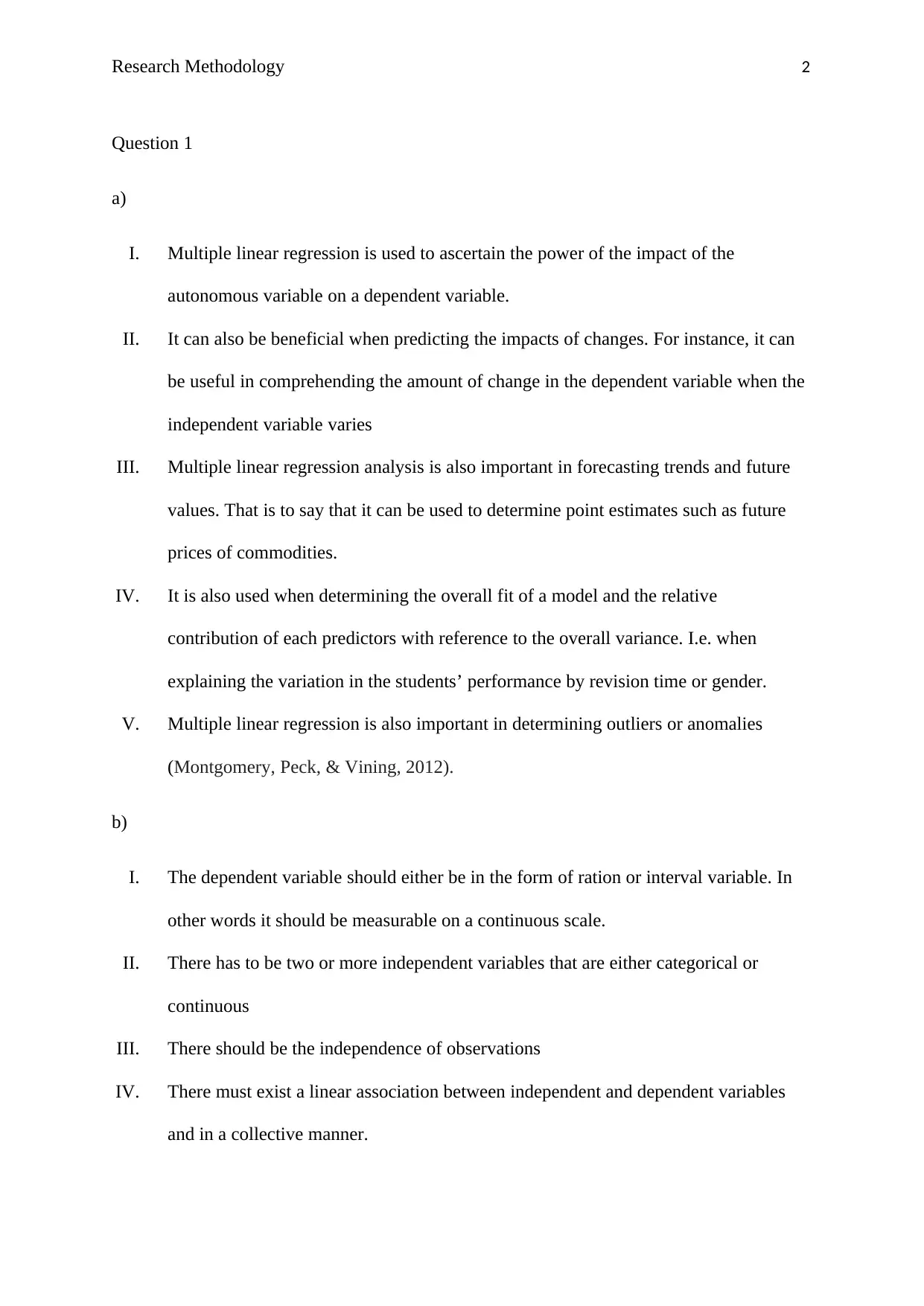
I. Multiple linear regression is used to ascertain the power of the impact of the
autonomous variable on a dependent variable.
II. It can also be beneficial when predicting the impacts of changes. For instance, it can
be useful in comprehending the amount of change in the dependent variable when the
independent variable varies
III. Multiple linear regression analysis is also important in forecasting trends and future
values. That is to say that it can be used to determine point estimates such as future
prices of commodities.
IV. It is also used when determining the overall fit of a model and the relative
contribution of each predictors with reference to the overall variance. I.e. when
explaining the variation in the students’ performance by revision time or gender.
V. Multiple linear regression is also important in determining outliers or anomalies
(Montgomery, Peck, & Vining, 2012).
b)
I. The dependent variable should either be in the form of ration or interval variable. In
other words it should be measurable on a continuous scale.
II. There has to be two or more independent variables that are either categorical or
continuous
III. There should be the independence of observations
IV. There must exist a linear association between independent and dependent variables
and in a collective manner.

Research Methodology 3
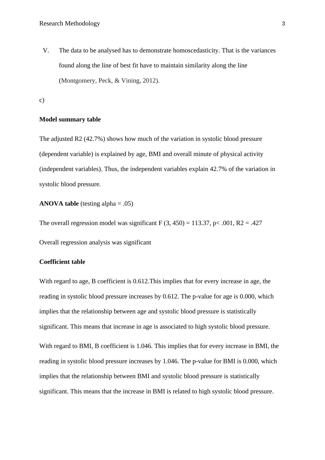
V. The data to be analysed has to demonstrate homoscedasticity. That is the variances
found along the line of best fit have to maintain similarity along the line
(Montgomery, Peck, & Vining, 2012).
c)
Model summary table
The adjusted R2 (42.7%) shows how much of the variation in systolic blood pressure
(dependent variable) is explained by age, BMI and overall minute of physical activity
(independent variables). Thus, the independent variables explain 42.7% of the variation in
systolic blood pressure.
ANOVA table (testing alpha = .05)
The overall regression model was significant F (3, 450) = 113.37, p< .001, R2 = .427
Overall regression analysis was significant
Coefficient table
With regard to age, B coefficient is 0.612.This implies that for every increase in age, the
reading in systolic blood pressure increases by 0.612. The p-value for age is 0.000, which
implies that the relationship between age and systolic blood pressure is statistically
significant. This means that increase in age is associated to high systolic blood pressure.
With regard to BMI, B coefficient is 1.046. This implies that for every increase in BMI, the
reading in systolic blood pressure increases by 1.046. The p-value for BMI is 0.000, which
implies that the relationship between BMI and systolic blood pressure is statistically
significant. This means that the increase in BMI is related to high systolic blood pressure.

Research Methodology 4
With regard to overall minute of PA, B coefficient is 0.001. This means that for every
increase in overall minute of PA, the reading in systolic blood pressure increases by 0.001.
The p-value for overall minute of PA is 0.270, which implies that the relationship between
overall minute of PA and systolic blood pressure is statistically insignificant. This means that
the increase in overall minute of PA is associated with low systolic blood pressure.
Multiple regression equation
Y = 74.86 + 0.61 (age) + 1.05 (BMI) – 0.01 (min PA).
Question 2
a)
I. Linearity – any independent variable have a linear association with the logit of the
resulting variable
II. Independent errors – this assumption indicates that errors shouldn’t be correlated for
two observations
III. Multi-collinearity – the independent variables should not be highly correlated with
one another.
IV. Homoscedasticity – the variance around the regression line is similar for all values of
x (predictor variable) (Yan & Su, 2009).
b)
I. Sex
II. Race
III. Age group
IV. Level of education (Kleinbaum, Kupper, Nizam, & Rosenberg, 2013).

Research Methodology 5
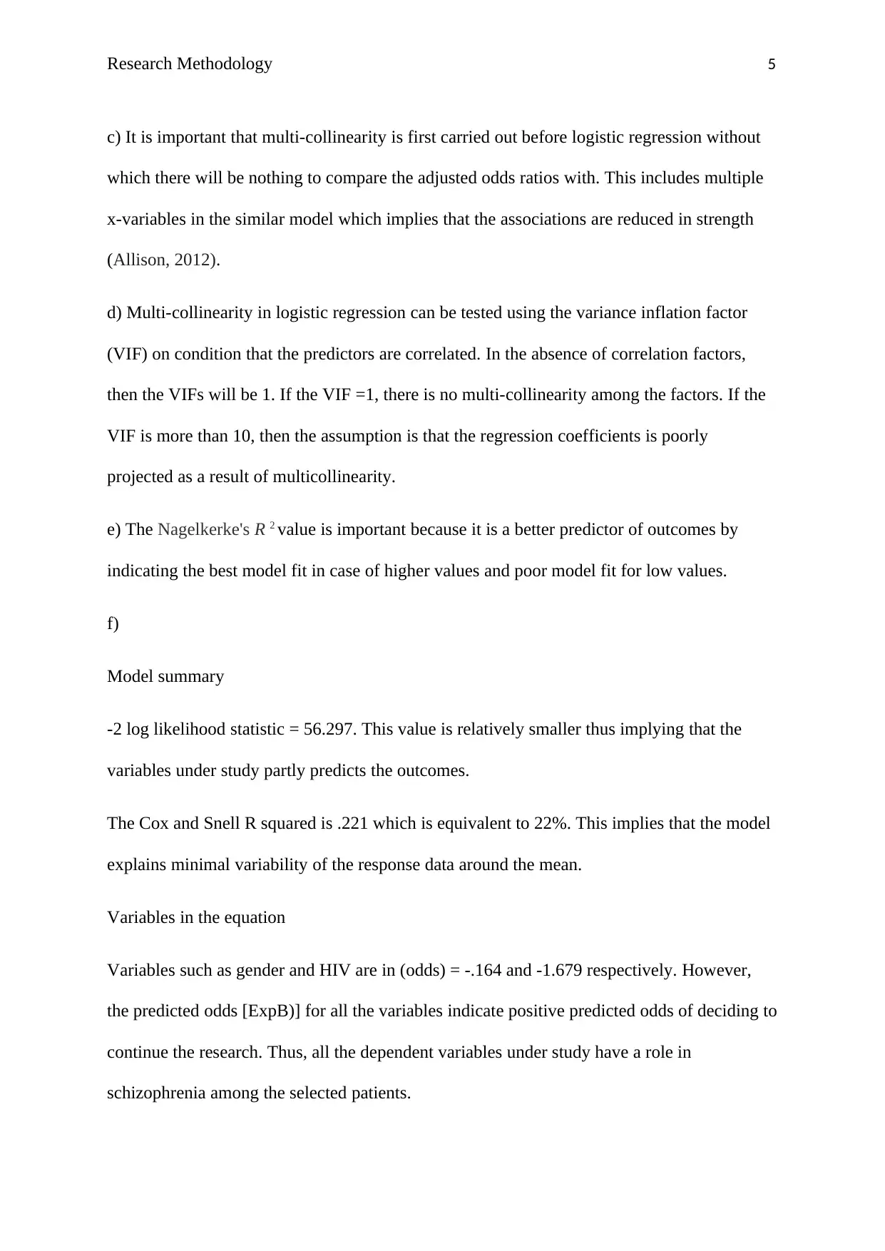
c) It is important that multi-collinearity is first carried out before logistic regression without
which there will be nothing to compare the adjusted odds ratios with. This includes multiple
x-variables in the similar model which implies that the associations are reduced in strength
(Allison, 2012).
d) Multi-collinearity in logistic regression can be tested using the variance inflation factor
(VIF) on condition that the predictors are correlated. In the absence of correlation factors,
then the VIFs will be 1. If the VIF =1, there is no multi-collinearity among the factors. If the
VIF is more than 10, then the assumption is that the regression coefficients is poorly
projected as a result of multicollinearity.
e) The Nagelkerke's R 2 value is important because it is a better predictor of outcomes by
indicating the best model fit in case of higher values and poor model fit for low values.
f)
Model summary
-2 log likelihood statistic = 56.297. This value is relatively smaller thus implying that the
variables under study partly predicts the outcomes.
The Cox and Snell R squared is .221 which is equivalent to 22%. This implies that the model
explains minimal variability of the response data around the mean.
Variables in the equation
Variables such as gender and HIV are in (odds) = -.164 and -1.679 respectively. However,
the predicted odds [ExpB)] for all the variables indicate positive predicted odds of deciding to
continue the research. Thus, all the dependent variables under study have a role in
schizophrenia among the selected patients.

Research Methodology 6
Question 3
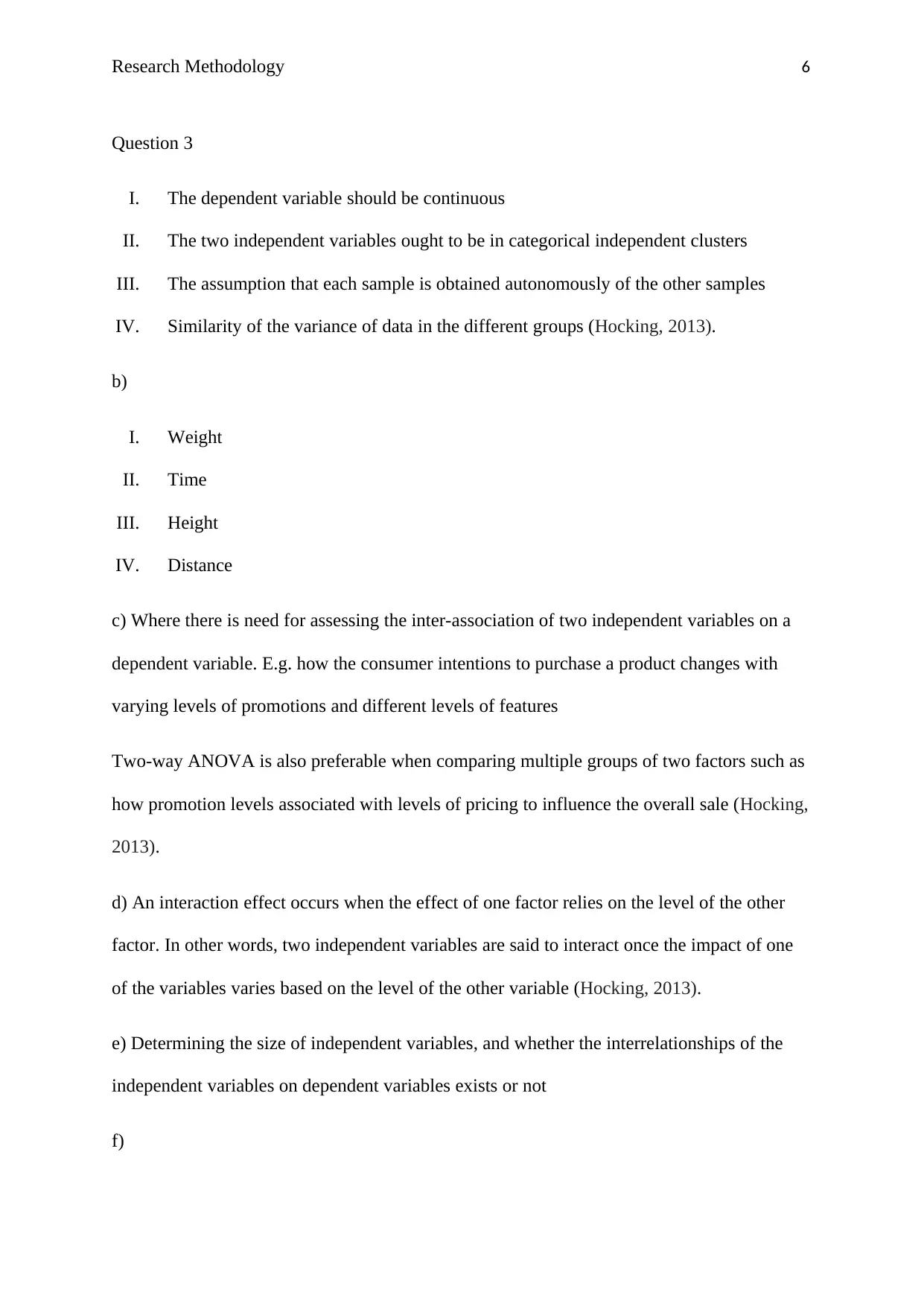
I. The dependent variable should be continuous
II. The two independent variables ought to be in categorical independent clusters
III. The assumption that each sample is obtained autonomously of the other samples
IV. Similarity of the variance of data in the different groups (Hocking, 2013).
b)
I. Weight
II. Time
III. Height
IV. Distance
c) Where there is need for assessing the inter-association of two independent variables on a
dependent variable. E.g. how the consumer intentions to purchase a product changes with
varying levels of promotions and different levels of features
Two-way ANOVA is also preferable when comparing multiple groups of two factors such as
how promotion levels associated with levels of pricing to influence the overall sale (Hocking,
2013).
d) An interaction effect occurs when the effect of one factor relies on the level of the other
factor. In other words, two independent variables are said to interact once the impact of one
of the variables varies based on the level of the other variable (Hocking, 2013).
e) Determining the size of independent variables, and whether the interrelationships of the
independent variables on dependent variables exists or not
f)

Research Methodology 7
The rows “gender”, “education level”, and “gender *education level” rows show whether
there is a statistically significant effect on the dependent variable (score in research methods
subjects). The p-value for gender is 0.9 which means there is a statistically insignificant
relation between gender and score in research methods subjects. The p-value for education
level is 0.01 which means that there is a statistically significant association between
education level and score in research methods subjects.
At p=0.04 level, there is a statistically significant interaction between the dependent (score in
research methods) and independent variables (gender and education level). Thus, the
interaction effect is significant. This implies that gender effect is significant when education
level is controlled.

Research Methodology 8
References
Allison, P. (2012). When can you safely ignore multicollinearity. Statistical Horizons, 5(1).
Hocking, R. R. (2013). Methods and applications of linear models: regression and the
analysis of variance. John Wiley & Sons.
Kleinbaum, D., Kupper, L., Nizam, A., & Rosenberg, E. (2013). Applied regression analysis
and other multivariable methods. Nelson Education.
Montgomery, D. C., Peck, E. A., & Vining, G. G. (2012). Introduction to linear regression
analysis (Vol. 821). John Wiley & Sons.
Yan, X., & Su, X. (2009). Linear regression analysis: theory and computing. World
Scientific.