Research Methods: Hypothesis Testing, T-Tests, and ANOVA Analysis

This assignment provides solutions to various hypothesis testing scenarios, including one-tailed and two-tailed tests. It covers t-tests, such as one-sample t-tests, paired sample t-tests, and independent samples t-tests, along with detailed data analysis and interpretations of p-values. The assignment also includes ANOVA and factorial ANOVA analyses to determine the statistical significance of different variables, such as body size and gender, on walking time. The decision to accept or reject null hypotheses is based on comparing p-values with the level of significance, providing a comprehensive overview of statistical analysis in research methods. Desklib offers a wide range of solved assignments and study resources to assist students in their academic endeavors.

Research methods 1
Student Name:
Student number:
Lecturer:

Research methods 2
PART ONE (HYPOTHESIS TESTING)
Question one
Scenario one: Do people in Winnipeg make more money than people living in the rest of
Canada?
The populations being compared here are people living in Winnipeg and the people living in the
rest of Canada.
Hypothesis test
H0: (Null hypothesis): People living in Winnipeg make the same amount of money people
living in the rest of Canada make.
H1: (Alternative hypothesis): People living in Winnipeg make more money than people living
in the rest of Canada.
The appropriate hypothesis for this test would be a one–tailed test since the alternative
hypothesis has given a one direction outcome. That is, people living in Winnipeg can only be
making MORE money THAN people living in the rest of Canada.
Scenario two: Do University of Manitoba students enrolled in Distance Education have different
GPAs than students enrolled in regular programs?
The populations being compared here are University of Manitoba students enrolled in regular
programs and those enrolled in distance education.
Hypothesis test
H0: (Null hypothesis): Students of University of Manitoba enrolled in Distance Education and
regular programs have equal GPAs.
H1: (Alternative hypothesis): Students of University of Manitoba enrolled in Distance
Education and regular programs have different GPAs.
The appropriate hypothesis for this test would be a two–tailed test since the alternative
hypothesis has given a two-sided impression possibility. That is, the students enrolled in distance
education could be having higher or lower GPAs than the regular students hence a two-tailed test
is used.
Scenario three: Do males laugh more than females?
The populations being compared here are males and females..

Research methods 3
Hypothesis test
H0: (Null hypothesis): Male and females laugh equally.
H1: (Alternative hypothesis): Males laugh more than females.
The appropriate hypothesis for this test would be a one–tailed test since the hypothesis has given
a direction to the outcome, that is, male laugh more than females.
Question two
Study A
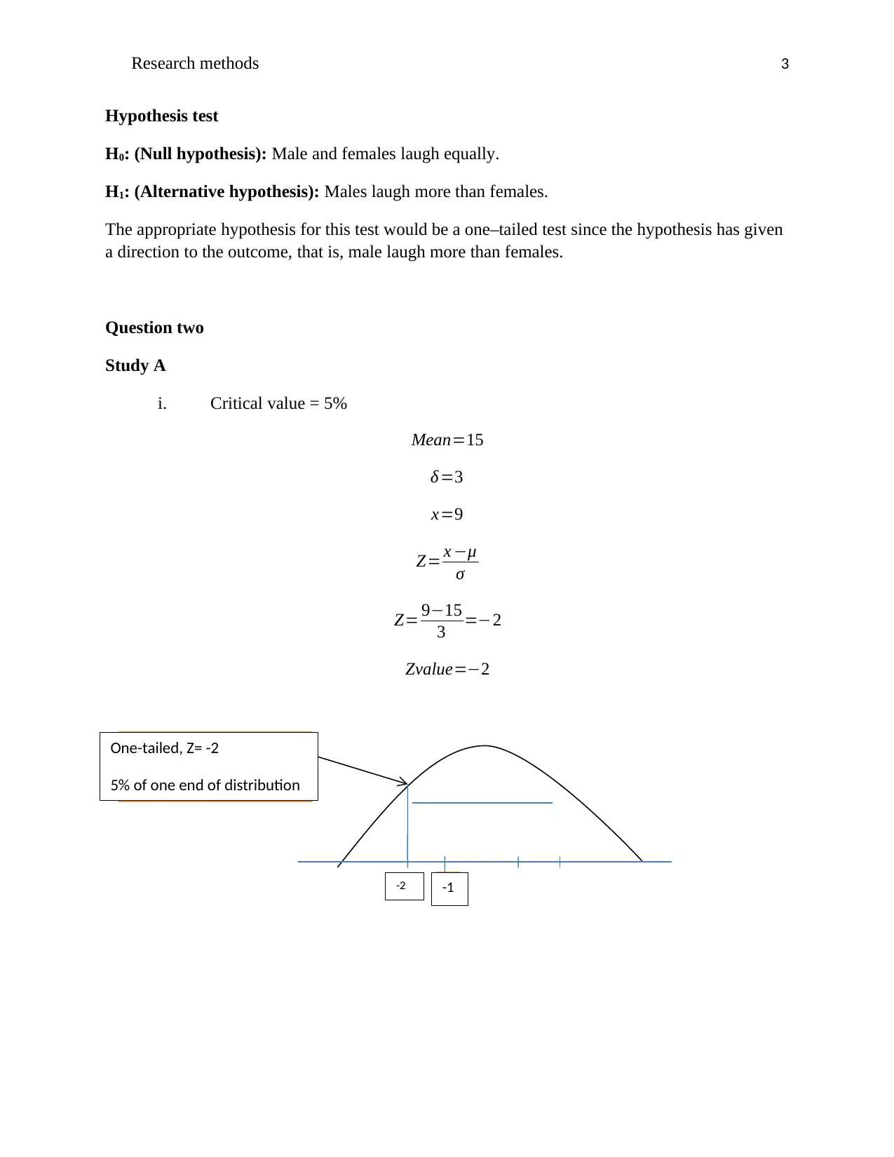
i. Critical value = 5%
Mean=15
δ =3
x=9
Z= x −μ
σ
Z= 9−15
3 =−2
Zvalue=−2
-2
One-tailed, Z= -2
5% of one end of distribution
-1

Research methods 4
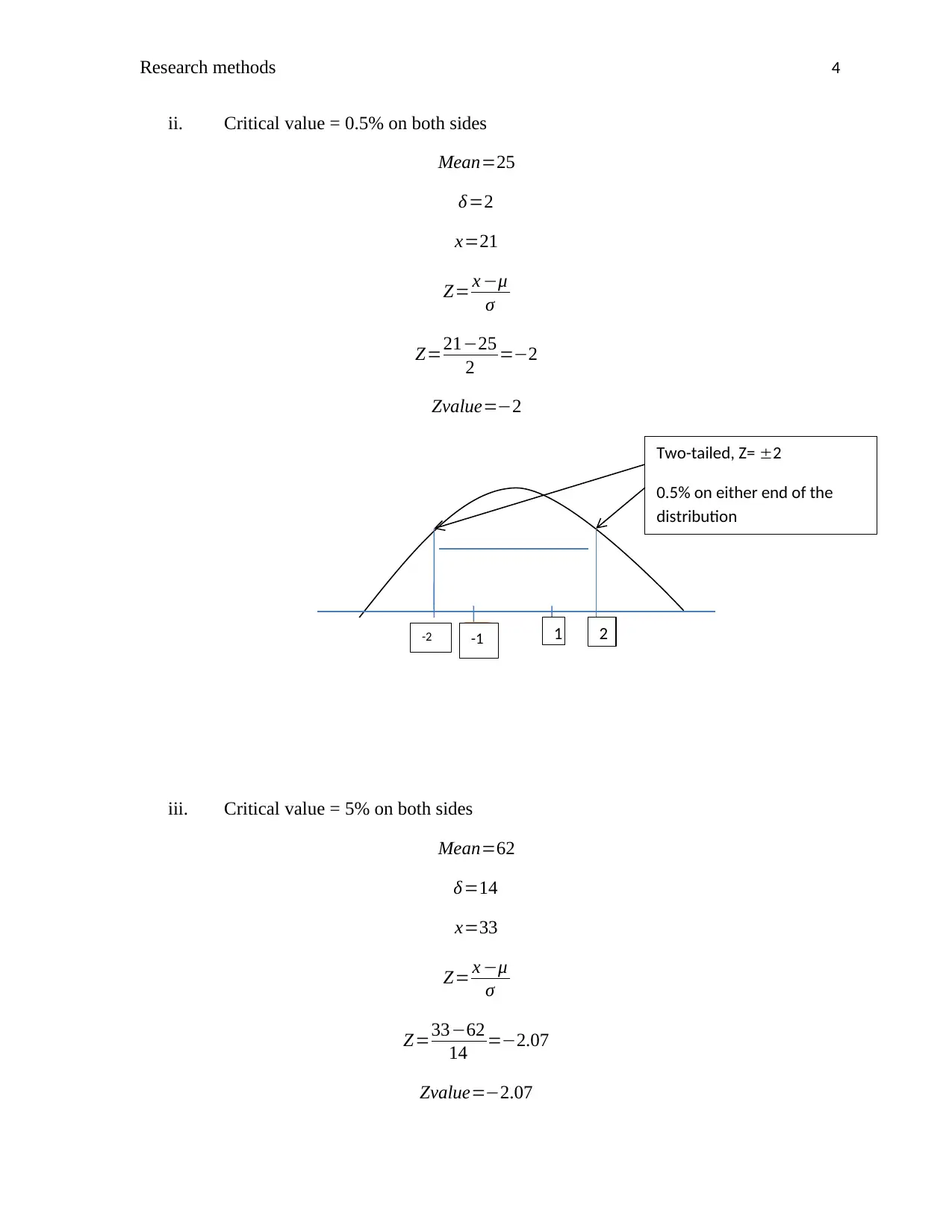
ii. Critical value = 0.5% on both sides
Mean=25
δ=2
x=21
Z= x −μ
σ
Z=21−25
2 =−2
Zvalue=−2
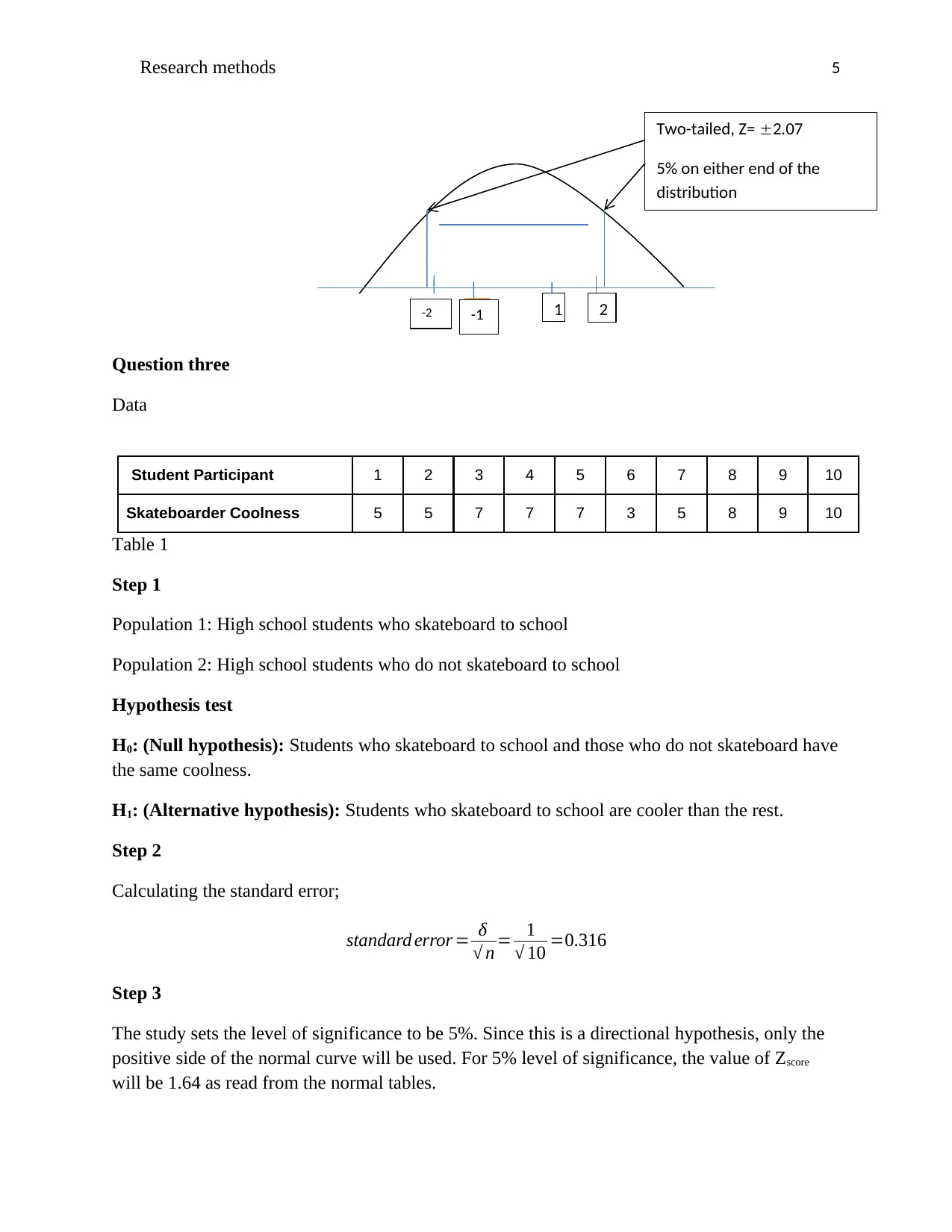
iii. Critical value = 5% on both sides
Mean=62
δ=14
x=33
Z= x −μ
σ
Z=33−62
14 =−2.07
Zvalue=−2.07
-2
Two-tailed, Z= 2
0.5% on either end of the
distribution
-1 1 2

Research methods 5
Question three
Data
Student Participant 1 2 3 4 5 6 7 8 9 10
Skateboarder Coolness 5 5 7 7 7 3 5 8 9 10
Table 1
Step 1
Population 1: High school students who skateboard to school
Population 2: High school students who do not skateboard to school
Hypothesis test
H0: (Null hypothesis): Students who skateboard to school and those who do not skateboard have
the same coolness.
H1: (Alternative hypothesis): Students who skateboard to school are cooler than the rest.
Step 2
Calculating the standard error;
standard error = δ
√ n = 1
√ 10 =0.316
Step 3
The study sets the level of significance to be 5%. Since this is a directional hypothesis, only the
positive side of the normal curve will be used. For 5% level of significance, the value of Zscore
will be 1.64 as read from the normal tables.
-2
Two-tailed, Z= 2.07
5% on either end of the
distribution
-1 1 2

Research methods 6
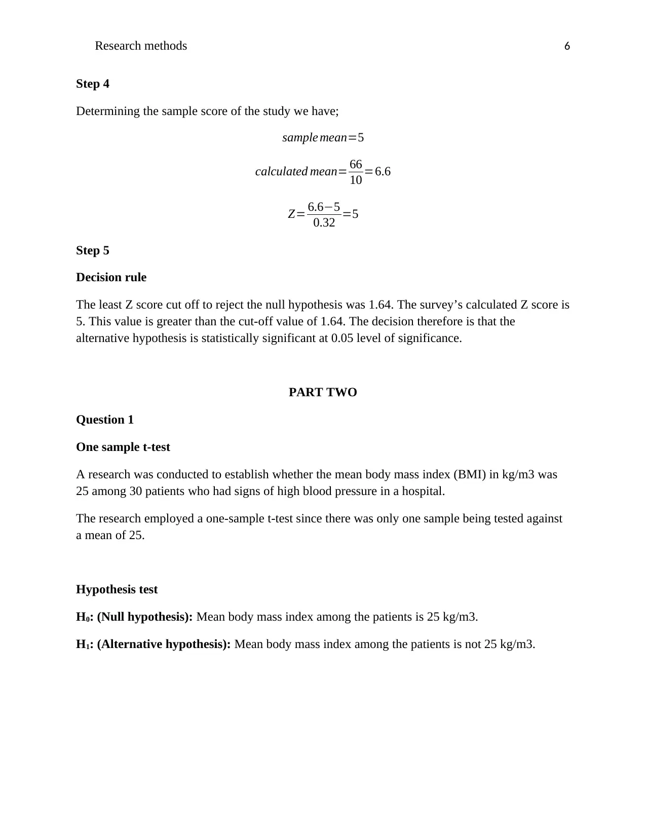
Step 4
Determining the sample score of the study we have;
sample mean=5
calculated mean= 66
10 =6.6
Z= 6.6−5
0.32 =5
Step 5
Decision rule
The least Z score cut off to reject the null hypothesis was 1.64. The survey’s calculated Z score is
5. This value is greater than the cut-off value of 1.64. The decision therefore is that the
alternative hypothesis is statistically significant at 0.05 level of significance.
PART TWO
Question 1
One sample t-test
A research was conducted to establish whether the mean body mass index (BMI) in kg/m3 was
25 among 30 patients who had signs of high blood pressure in a hospital.
The research employed a one-sample t-test since there was only one sample being tested against
a mean of 25.
Hypothesis test
H0: (Null hypothesis): Mean body mass index among the patients is 25 kg/m3.
H1: (Alternative hypothesis): Mean body mass index among the patients is not 25 kg/m3.

Research methods 7
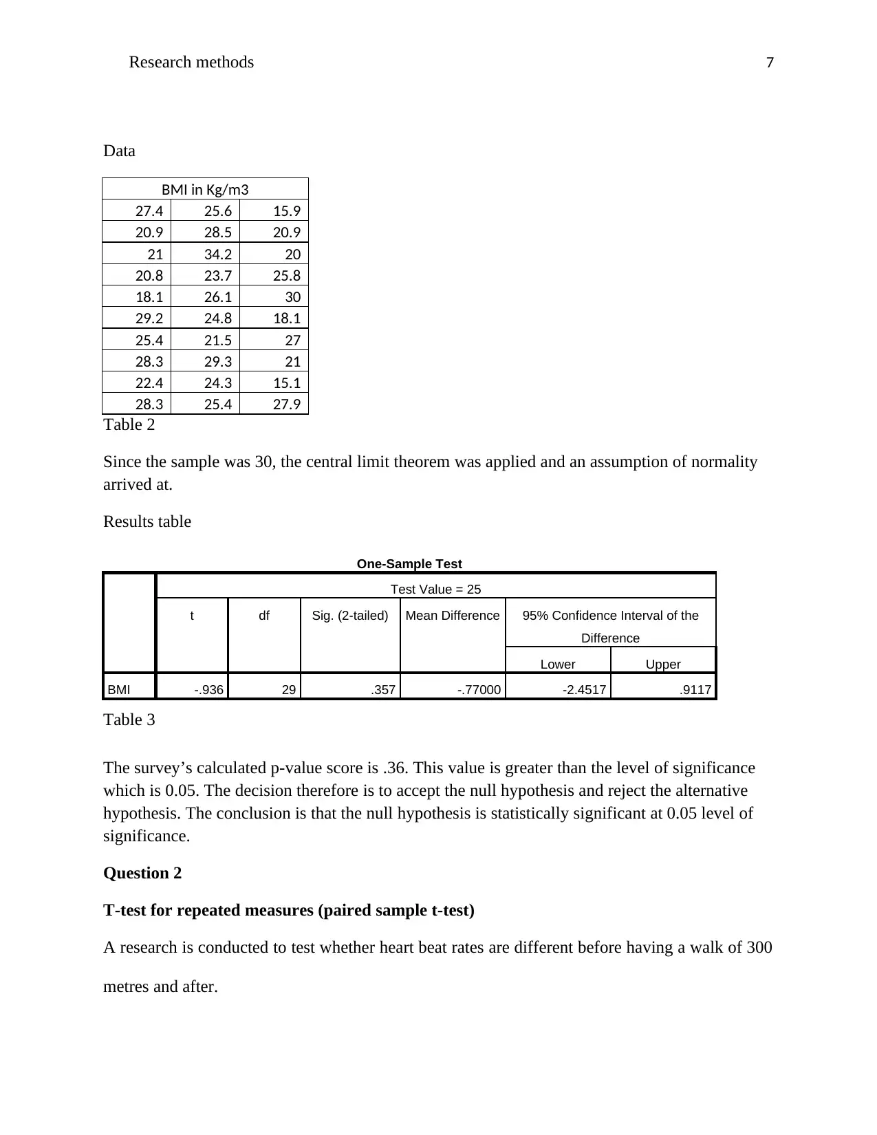
Data
BMI in Kg/m3
27.4 25.6 15.9
20.9 28.5 20.9
21 34.2 20
20.8 23.7 25.8
18.1 26.1 30
29.2 24.8 18.1
25.4 21.5 27
28.3 29.3 21
22.4 24.3 15.1
28.3 25.4 27.9
Table 2
Since the sample was 30, the central limit theorem was applied and an assumption of normality
arrived at.
Results table
One-Sample Test
Test Value = 25
t df Sig. (2-tailed) Mean Difference 95% Confidence Interval of the
Difference
Lower Upper
BMI -.936 29 .357 -.77000 -2.4517 .9117
Table 3
The survey’s calculated p-value score is .36. This value is greater than the level of significance
which is 0.05. The decision therefore is to accept the null hypothesis and reject the alternative
hypothesis. The conclusion is that the null hypothesis is statistically significant at 0.05 level of
significance.
Question 2
T-test for repeated measures (paired sample t-test)
A research is conducted to test whether heart beat rates are different before having a walk of 300
metres and after.

Research methods 8
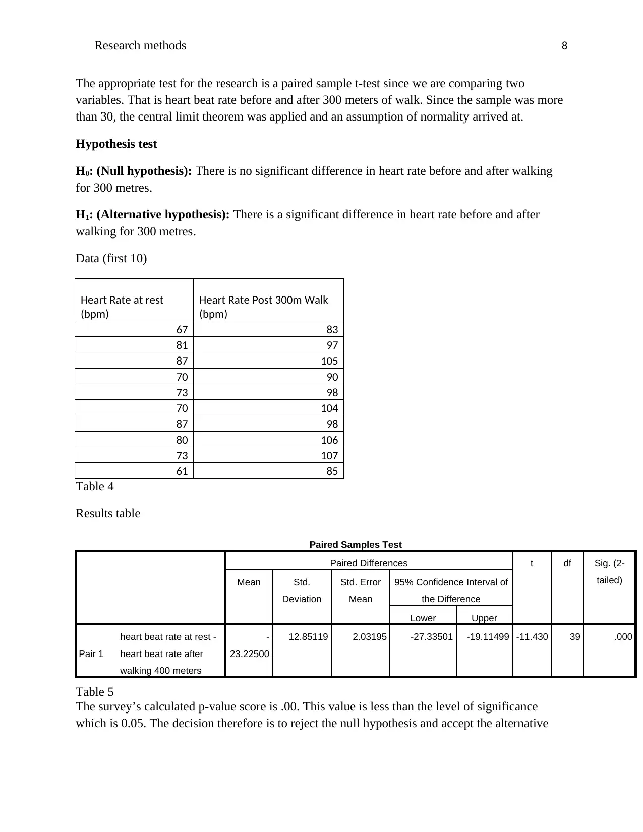
The appropriate test for the research is a paired sample t-test since we are comparing two
variables. That is heart beat rate before and after 300 meters of walk. Since the sample was more
than 30, the central limit theorem was applied and an assumption of normality arrived at.
Hypothesis test
H0: (Null hypothesis): There is no significant difference in heart rate before and after walking
for 300 metres.
H1: (Alternative hypothesis): There is a significant difference in heart rate before and after
walking for 300 metres.
Data (first 10)
Heart Rate at rest
(bpm)
Heart Rate Post 300m Walk
(bpm)
67 83
81 97
87 105
70 90
73 98
70 104
87 98
80 106
73 107
61 85
Table 4
Results table
Paired Samples Test
Paired Differences t df Sig. (2-
tailed)Mean Std.
Deviation
Std. Error
Mean
95% Confidence Interval of
the Difference
Lower Upper
Pair 1
heart beat rate at rest -
heart beat rate after
walking 400 meters
-
23.22500
12.85119 2.03195 -27.33501 -19.11499 -11.430 39 .000
Table 5
The survey’s calculated p-value score is .00. This value is less than the level of significance
which is 0.05. The decision therefore is to reject the null hypothesis and accept the alternative

Research methods 9
hypothesis. The conclusion is that the alternative hypothesis is statistically significant at 0.05
level of significance.
Question 3
Independent sample t-test
A sample of 46 intern accountants employed in a bank had been trained differently. The first 23
had gone through PC- based training while the other 23 went through traditional lectures. The
human resources department wanted to establish whether there is a significant difference in their
mean aptitude scores.
The appropriate test was an independent samples t-test since the two samples are independent.
They have been drawn from different populations.
Since the sample was drawn from a normally distributed population an assumption of normality
was arrived at.
Hypothesis test
H0: (Null hypothesis): There is no difference in mean aptitude test scores between the two
groups.
H1: (Alternative hypothesis): There is a significant difference in mean aptitude test scores
between the two groups.

Research methods 10
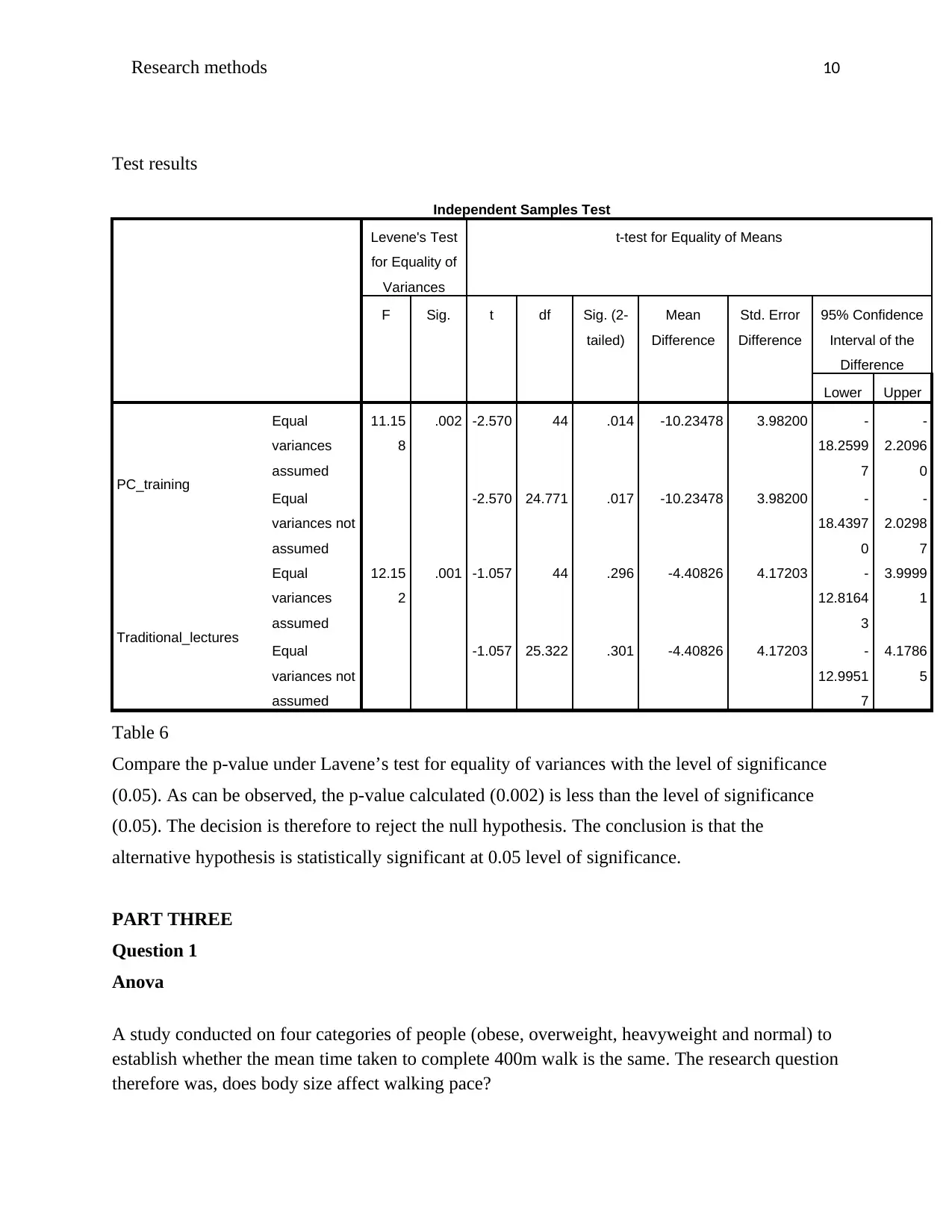
Test results
Independent Samples Test
Levene's Test
for Equality of
Variances
t-test for Equality of Means
F Sig. t df Sig. (2-
tailed)
Mean
Difference
Std. Error
Difference
95% Confidence
Interval of the
Difference
Lower Upper
PC_training
Equal
variances
assumed
11.15
8
.002 -2.570 44 .014 -10.23478 3.98200 -
18.2599
7
-
2.2096
0
Equal
variances not
assumed
-2.570 24.771 .017 -10.23478 3.98200 -
18.4397
0
-
2.0298
7
Traditional_lectures
Equal
variances
assumed
12.15
2
.001 -1.057 44 .296 -4.40826 4.17203 -
12.8164
3
3.9999
1
Equal
variances not
assumed
-1.057 25.322 .301 -4.40826 4.17203 -
12.9951
7
4.1786
5
Table 6
Compare the p-value under Lavene’s test for equality of variances with the level of significance
(0.05). As can be observed, the p-value calculated (0.002) is less than the level of significance
(0.05). The decision is therefore to reject the null hypothesis. The conclusion is that the
alternative hypothesis is statistically significant at 0.05 level of significance.
PART THREE
Question 1
Anova
A study conducted on four categories of people (obese, overweight, heavyweight and normal) to
establish whether the mean time taken to complete 400m walk is the same. The research question
therefore was, does body size affect walking pace?

Research methods 11
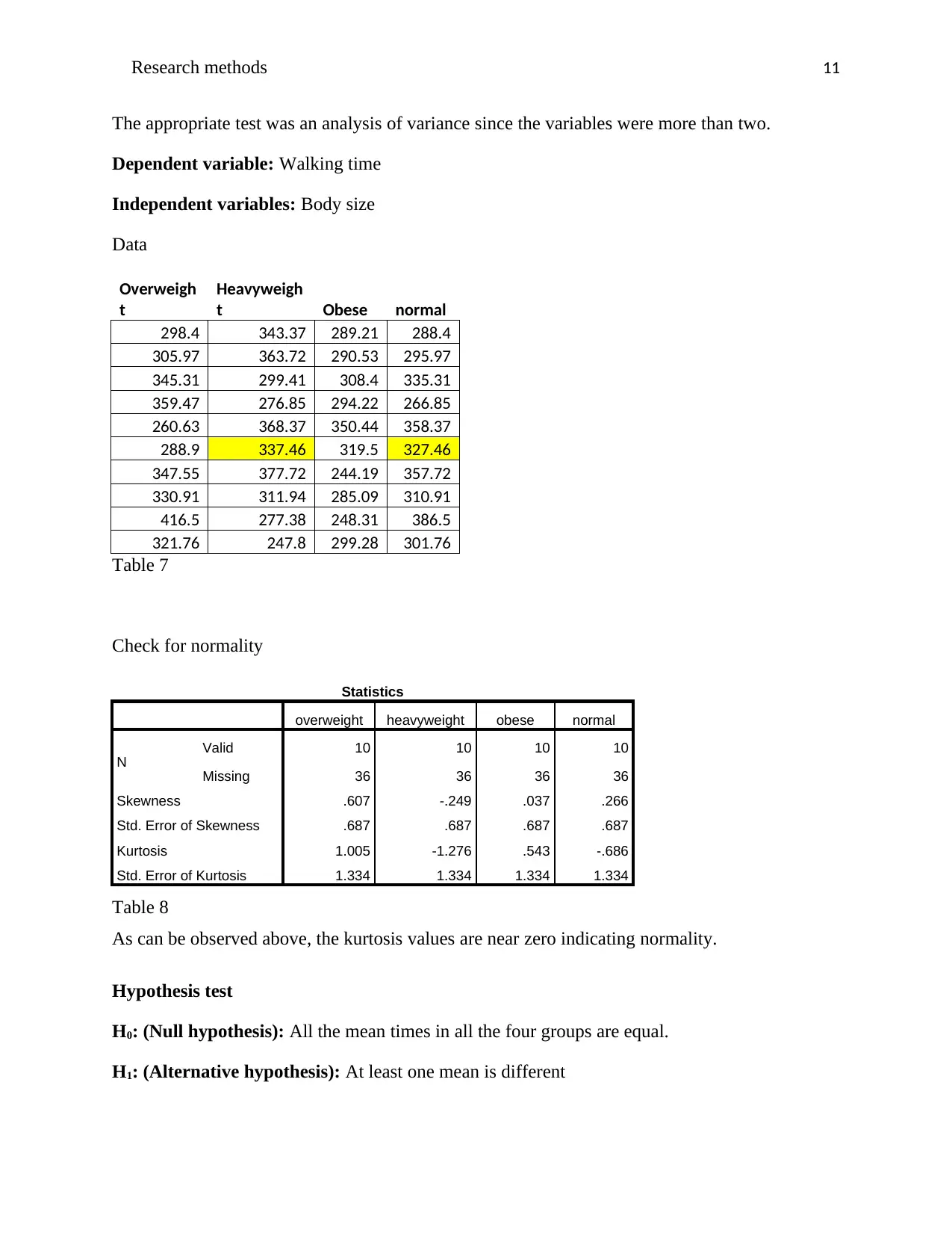
The appropriate test was an analysis of variance since the variables were more than two.
Dependent variable: Walking time
Independent variables: Body size
Data
Overweigh
t
Heavyweigh
t Obese normal
298.4 343.37 289.21 288.4
305.97 363.72 290.53 295.97
345.31 299.41 308.4 335.31
359.47 276.85 294.22 266.85
260.63 368.37 350.44 358.37
288.9 337.46 319.5 327.46
347.55 377.72 244.19 357.72
330.91 311.94 285.09 310.91
416.5 277.38 248.31 386.5
321.76 247.8 299.28 301.76
Table 7
Check for normality
Statistics
overweight heavyweight obese normal
N Valid 10 10 10 10
Missing 36 36 36 36
Skewness .607 -.249 .037 .266
Std. Error of Skewness .687 .687 .687 .687
Kurtosis 1.005 -1.276 .543 -.686
Std. Error of Kurtosis 1.334 1.334 1.334 1.334
Table 8
As can be observed above, the kurtosis values are near zero indicating normality.
Hypothesis test
H0: (Null hypothesis): All the mean times in all the four groups are equal.
H1: (Alternative hypothesis): At least one mean is different

Research methods 12
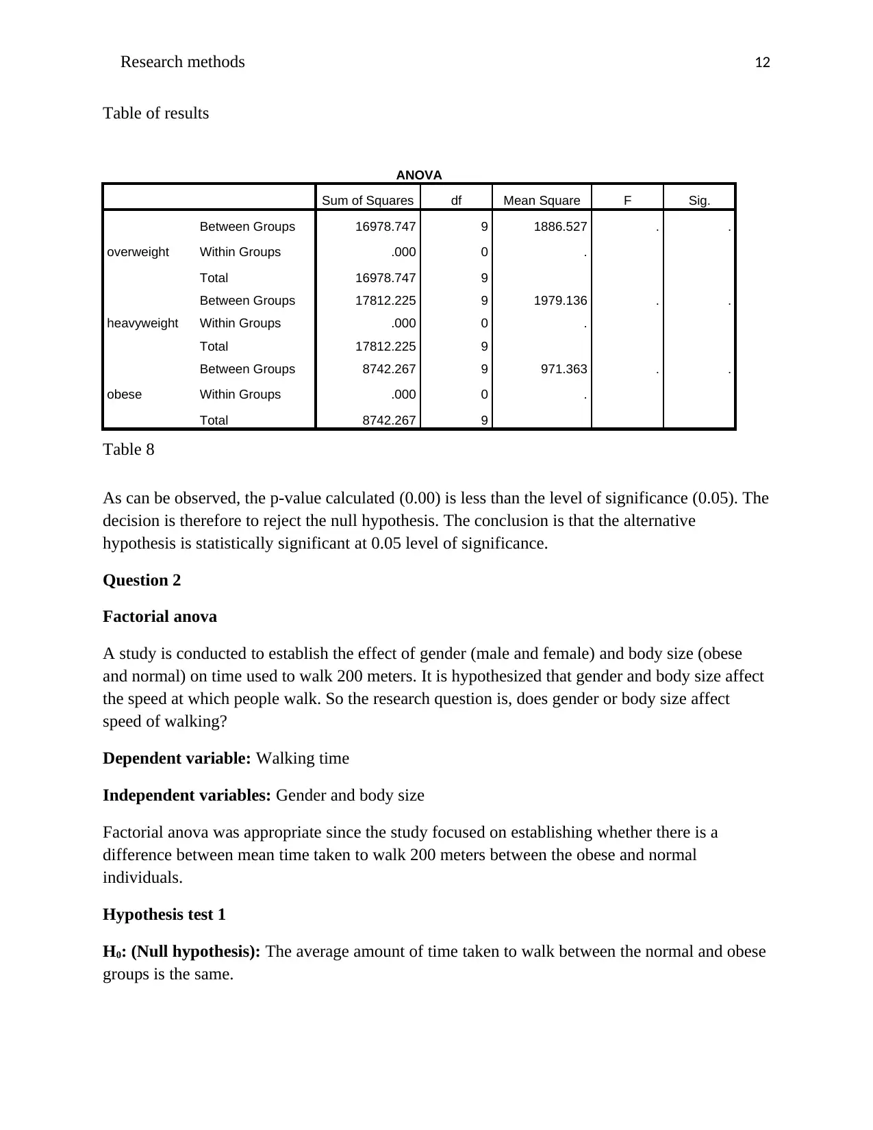
Table of results
ANOVA
Sum of Squares df Mean Square F Sig.
overweight
Between Groups 16978.747 9 1886.527 . .
Within Groups .000 0 .
Total 16978.747 9
heavyweight
Between Groups 17812.225 9 1979.136 . .
Within Groups .000 0 .
Total 17812.225 9
obese
Between Groups 8742.267 9 971.363 . .
Within Groups .000 0 .
Total 8742.267 9
Table 8
As can be observed, the p-value calculated (0.00) is less than the level of significance (0.05). The
decision is therefore to reject the null hypothesis. The conclusion is that the alternative
hypothesis is statistically significant at 0.05 level of significance.
Question 2
Factorial anova
A study is conducted to establish the effect of gender (male and female) and body size (obese
and normal) on time used to walk 200 meters. It is hypothesized that gender and body size affect
the speed at which people walk. So the research question is, does gender or body size affect
speed of walking?
Dependent variable: Walking time
Independent variables: Gender and body size
Factorial anova was appropriate since the study focused on establishing whether there is a
difference between mean time taken to walk 200 meters between the obese and normal
individuals.
Hypothesis test 1
H0: (Null hypothesis): The average amount of time taken to walk between the normal and obese
groups is the same.