Research Methods

This document provides study material on Research Methods including regression analysis, tests for weak form efficiency, and empirical discussions. It also includes descriptive statistics and model summary. Find solved assignments, essays, and dissertations on Research Methods at Desklib.

Running head: Research Methods
Research Methods
Name of the Student
Course Id:
Course Name:

1
Research Methods
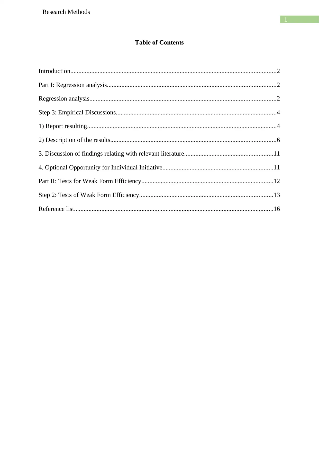
Table of Contents
Introduction................................................................................................................................2
Part I: Regression analysis.........................................................................................................2
Regression analysis....................................................................................................................2
Step 3: Empirical Discussions....................................................................................................4
1) Report resulting......................................................................................................................4
2) Description of the results.......................................................................................................6
3. Discussion of findings relating with relevant literature.......................................................11
4. Optional Opportunity for Individual Initiative.....................................................................11
Part II: Tests for Weak Form Efficiency..................................................................................12
Step 2: Tests of Weak Form Efficiency...................................................................................13
Reference list............................................................................................................................16

2
Research Methods
Introduction
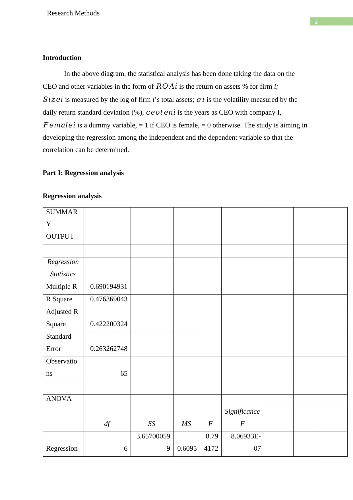
In the above diagram, the statistical analysis has been done taking the data on the
CEO and other variables in the form of 𝑅𝑂𝐴𝑖 is the return on assets % for firm i;
𝑆𝑖𝑧𝑒𝑖 is measured by the log of firm i’s total assets; 𝜎𝑖 is the volatility measured by the
daily return standard deviation (%), 𝑐𝑒𝑜𝑡𝑒𝑛𝑖 is the years as CEO with company I,
𝐹𝑒𝑚𝑎𝑙𝑒𝑖 is a dummy variable, = 1 if CEO is female, = 0 otherwise. The study is aiming in
developing the regression among the independent and the dependent variable so that the
correlation can be determined.
Part I: Regression analysis
Regression analysis
SUMMAR
Y
OUTPUT
Regression
Statistics
Multiple R 0.690194931
R Square 0.476369043
Adjusted R
Square 0.422200324
Standard
Error 0.263262748
Observatio
ns 65
ANOVA
df SS MS F
Significance
F
Regression 6
3.65700059
9 0.6095
8.79
4172
8.06933E-
07

3
Research Methods
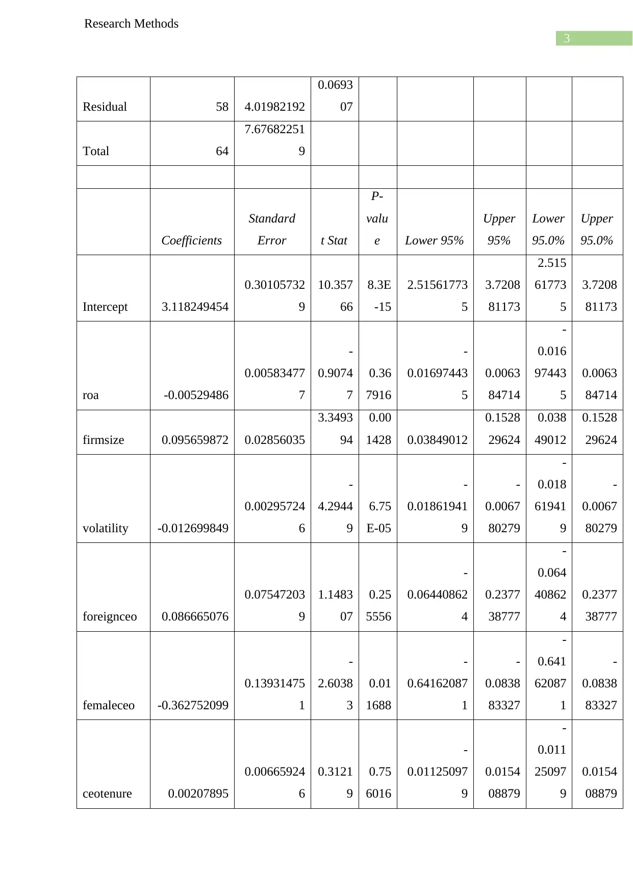
Residual 58 4.01982192
0.0693
07
Total 64
7.67682251
9
Coefficients
Standard
Error t Stat
P-
valu
e Lower 95%
Upper
95%
Lower
95.0%
Upper
95.0%
Intercept 3.118249454
0.30105732
9
10.357
66
8.3E
-15
2.51561773
5
3.7208
81173
2.515
61773
5
3.7208
81173
roa -0.00529486
0.00583477
7
-
0.9074
7
0.36
7916
-
0.01697443
5
0.0063
84714
-
0.016
97443
5
0.0063
84714
firmsize 0.095659872 0.02856035
3.3493
94
0.00
1428 0.03849012
0.1528
29624
0.038
49012
0.1528
29624
volatility -0.012699849
0.00295724
6
-
4.2944
9
6.75
E-05
-
0.01861941
9
-
0.0067
80279
-
0.018
61941
9
-
0.0067
80279
foreignceo 0.086665076
0.07547203
9
1.1483
07
0.25
5556
-
0.06440862
4
0.2377
38777
-
0.064
40862
4
0.2377
38777
femaleceo -0.362752099
0.13931475
1
-
2.6038
3
0.01
1688
-
0.64162087
1
-
0.0838
83327
-
0.641
62087
1
-
0.0838
83327
ceotenure 0.00207895
0.00665924
6
0.3121
9
0.75
6016
-
0.01125097
9
0.0154
08879
-
0.011
25097
9
0.0154
08879

4
Research Methods
Table 1: Regression analysis
Step 3: Empirical Discussions
The required regression equation that has been used for this purpose of development
of better description of the model is
𝑌𝑖=𝛼+𝛽1𝑅𝑂𝐴𝑖+𝛽2𝑆𝑖𝑧𝑒𝑖+𝛽3𝜎𝑖+𝛽4𝑐𝑒𝑜𝑡𝑒𝑛𝑖+𝛽5𝐹𝑒𝑚𝑎𝑙𝑒𝑖+𝛽6𝐹𝑜𝑟𝑒𝑖𝑔𝑛𝑖+𝜀𝑖
where: 𝑌𝑖 is the log salary for CEO i; 𝑅𝑂𝐴𝑖 is the return on assets % for firm i; 𝑆𝑖𝑧𝑒𝑖 is
measured by the log of firm i’s total assets; 𝜎𝑖 is the volatility measured by the daily return
standard deviation (%);
𝑐𝑒𝑜𝑡𝑒𝑛𝑖 is the years as CEO with company i; 𝐹𝑒𝑚𝑎𝑙𝑒𝑖 is a dummy variable, = 1 if CEO
is female, = 0 otherwise. 𝐹𝑜𝑟𝑒𝑖𝑔𝑛𝑖 is a dummy variable, = 1 if CEO is foreign, 0
otherwise.
1) Report resulting
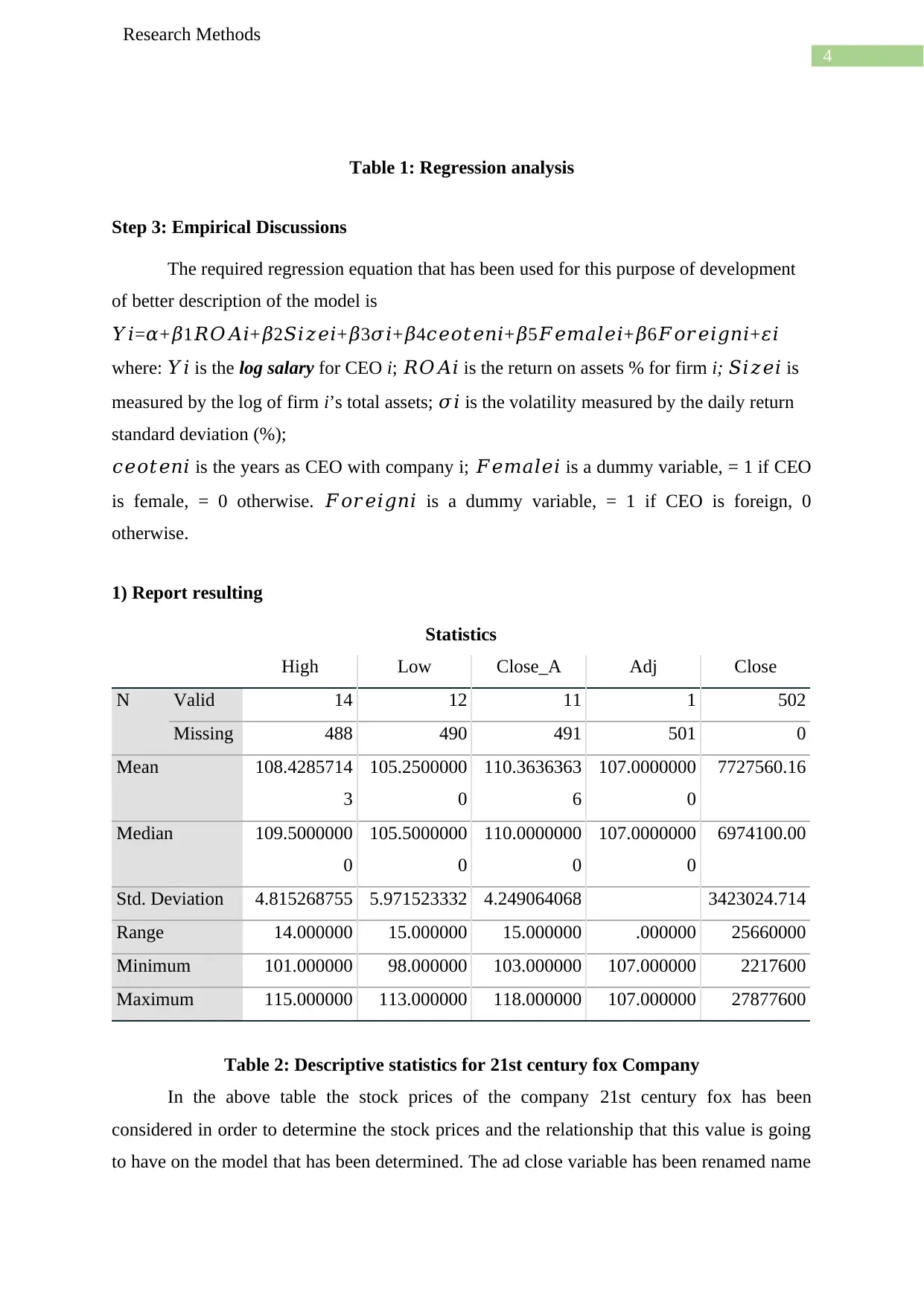
Statistics
High Low Close_A Adj Close
N Valid 14 12 11 1 502
Missing 488 490 491 501 0
Mean 108.4285714
3
105.2500000
0
110.3636363
6
107.0000000
0
7727560.16
Median 109.5000000
0
105.5000000
0
110.0000000
0
107.0000000
0
6974100.00
Std. Deviation 4.815268755 5.971523332 4.249064068 3423024.714
Range 14.000000 15.000000 15.000000 .000000 25660000
Minimum 101.000000 98.000000 103.000000 107.000000 2217600
Maximum 115.000000 113.000000 118.000000 107.000000 27877600
Table 2: Descriptive statistics for 21st century fox Company
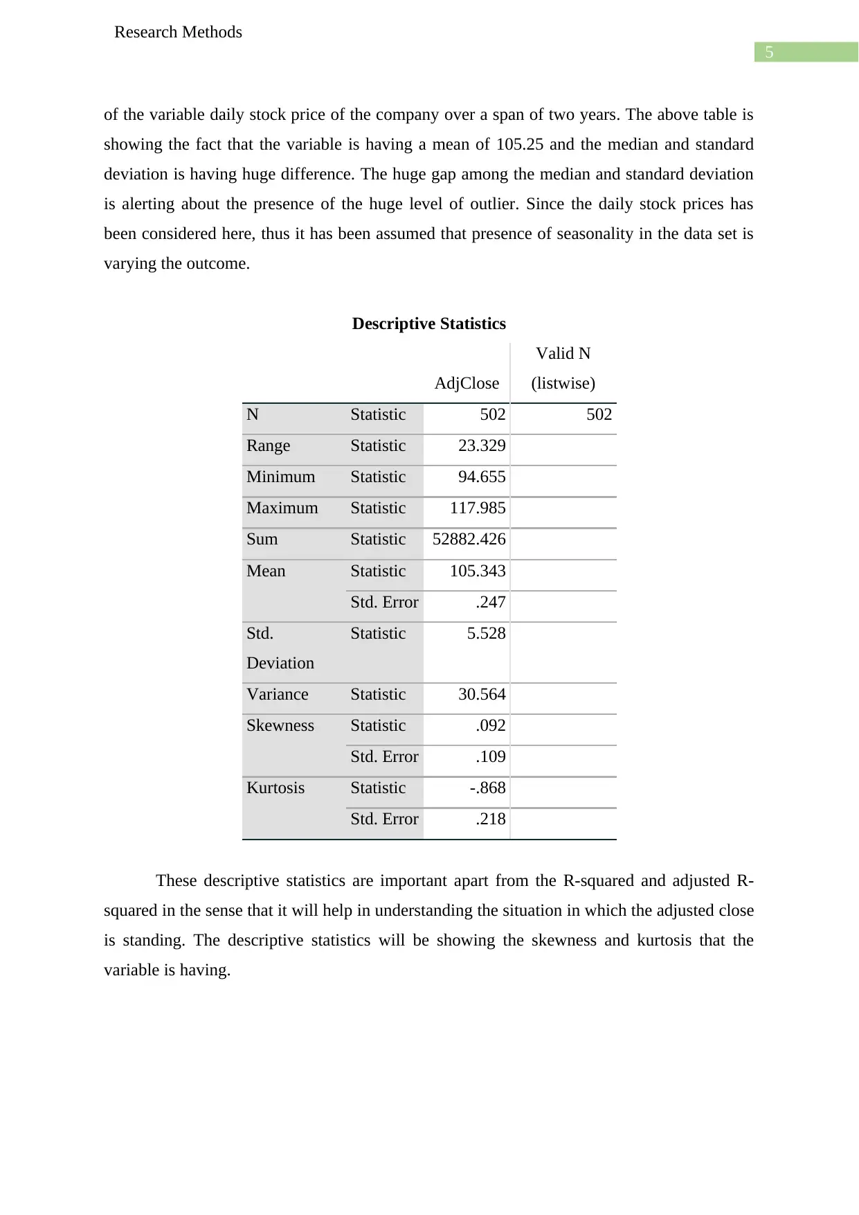
In the above table the stock prices of the company 21st century fox has been
considered in order to determine the stock prices and the relationship that this value is going
to have on the model that has been determined. The ad close variable has been renamed name

5
Research Methods
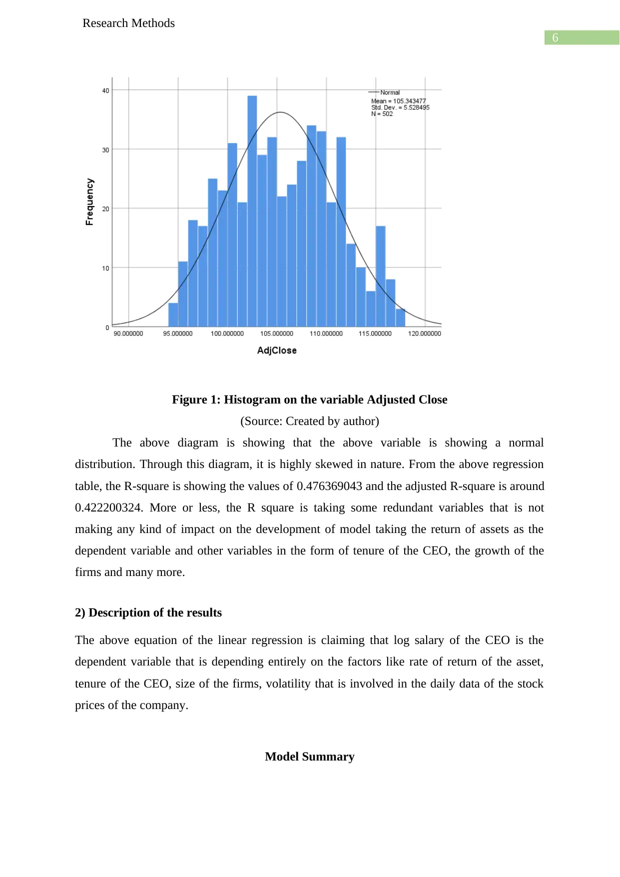
of the variable daily stock price of the company over a span of two years. The above table is
showing the fact that the variable is having a mean of 105.25 and the median and standard
deviation is having huge difference. The huge gap among the median and standard deviation
is alerting about the presence of the huge level of outlier. Since the daily stock prices has
been considered here, thus it has been assumed that presence of seasonality in the data set is
varying the outcome.
Descriptive Statistics
AdjClose
Valid N
(listwise)
N Statistic 502 502
Range Statistic 23.329
Minimum Statistic 94.655
Maximum Statistic 117.985
Sum Statistic 52882.426
Mean Statistic 105.343
Std. Error .247
Std.
Deviation
Statistic 5.528
Variance Statistic 30.564
Skewness Statistic .092
Std. Error .109
Kurtosis Statistic -.868
Std. Error .218
These descriptive statistics are important apart from the R-squared and adjusted R-
squared in the sense that it will help in understanding the situation in which the adjusted close
is standing. The descriptive statistics will be showing the skewness and kurtosis that the
variable is having.

6
Research Methods
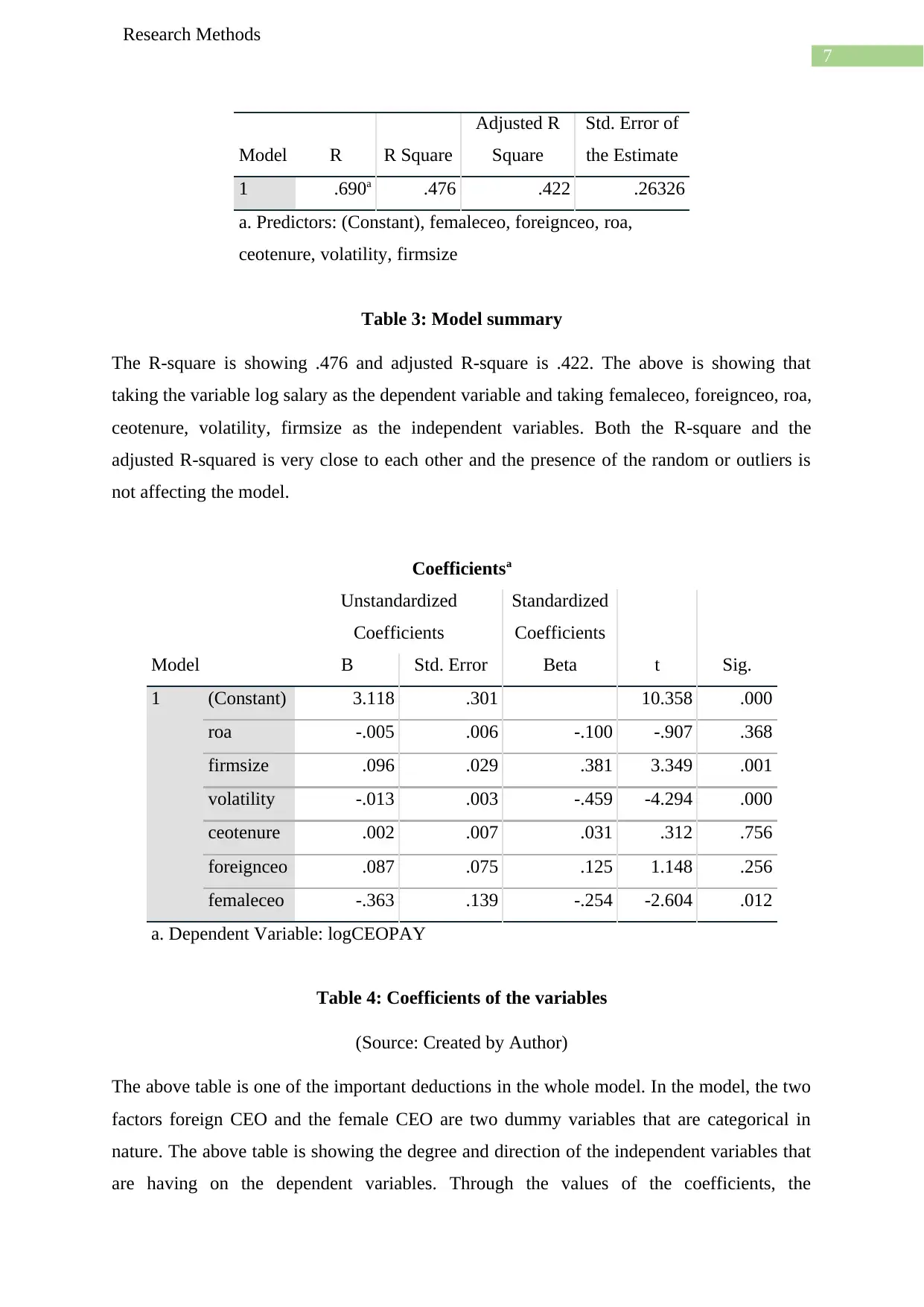
Figure 1: Histogram on the variable Adjusted Close
(Source: Created by author)
The above diagram is showing that the above variable is showing a normal
distribution. Through this diagram, it is highly skewed in nature. From the above regression
table, the R-square is showing the values of 0.476369043 and the adjusted R-square is around
0.422200324. More or less, the R square is taking some redundant variables that is not
making any kind of impact on the development of model taking the return of assets as the
dependent variable and other variables in the form of tenure of the CEO, the growth of the
firms and many more.
2) Description of the results
The above equation of the linear regression is claiming that log salary of the CEO is the
dependent variable that is depending entirely on the factors like rate of return of the asset,
tenure of the CEO, size of the firms, volatility that is involved in the daily data of the stock
prices of the company.
Model Summary

7
Research Methods
Model R R Square
Adjusted R
Square
Std. Error of
the Estimate
1 .690a .476 .422 .26326
a. Predictors: (Constant), femaleceo, foreignceo, roa,
ceotenure, volatility, firmsize
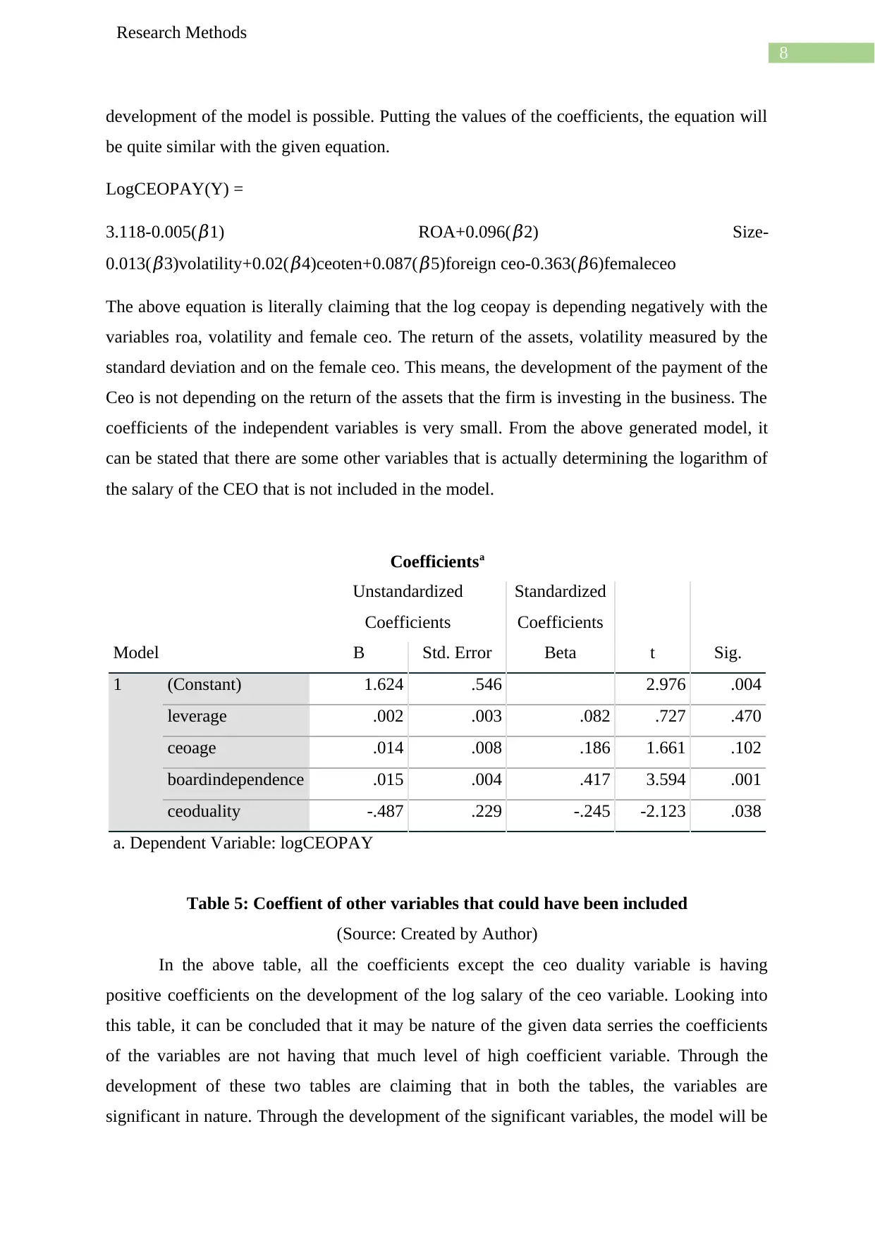
Table 3: Model summary
The R-square is showing .476 and adjusted R-square is .422. The above is showing that
taking the variable log salary as the dependent variable and taking femaleceo, foreignceo, roa,
ceotenure, volatility, firmsize as the independent variables. Both the R-square and the
adjusted R-squared is very close to each other and the presence of the random or outliers is
not affecting the model.
Coefficientsa
Model
Unstandardized
Coefficients
Standardized
Coefficients
t Sig.B Std. Error Beta
1 (Constant) 3.118 .301 10.358 .000
roa -.005 .006 -.100 -.907 .368
firmsize .096 .029 .381 3.349 .001
volatility -.013 .003 -.459 -4.294 .000
ceotenure .002 .007 .031 .312 .756
foreignceo .087 .075 .125 1.148 .256
femaleceo -.363 .139 -.254 -2.604 .012
a. Dependent Variable: logCEOPAY
Table 4: Coefficients of the variables
(Source: Created by Author)
The above table is one of the important deductions in the whole model. In the model, the two
factors foreign CEO and the female CEO are two dummy variables that are categorical in
nature. The above table is showing the degree and direction of the independent variables that
are having on the dependent variables. Through the values of the coefficients, the

8
Research Methods
development of the model is possible. Putting the values of the coefficients, the equation will
be quite similar with the given equation.
LogCEOPAY(Y) =
3.118-0.005(𝛽1) ROA+0.096(𝛽2) Size-
0.013(𝛽3)volatility+0.02(𝛽4)ceoten+0.087(𝛽5)foreign ceo-0.363(𝛽6)femaleceo
The above equation is literally claiming that the log ceopay is depending negatively with the
variables roa, volatility and female ceo. The return of the assets, volatility measured by the
standard deviation and on the female ceo. This means, the development of the payment of the
Ceo is not depending on the return of the assets that the firm is investing in the business. The
coefficients of the independent variables is very small. From the above generated model, it
can be stated that there are some other variables that is actually determining the logarithm of
the salary of the CEO that is not included in the model.
Coefficientsa
Model
Unstandardized
Coefficients
Standardized
Coefficients
t Sig.B Std. Error Beta
1 (Constant) 1.624 .546 2.976 .004
leverage .002 .003 .082 .727 .470
ceoage .014 .008 .186 1.661 .102
boardindependence .015 .004 .417 3.594 .001
ceoduality -.487 .229 -.245 -2.123 .038
a. Dependent Variable: logCEOPAY
Table 5: Coeffient of other variables that could have been included
(Source: Created by Author)
In the above table, all the coefficients except the ceo duality variable is having
positive coefficients on the development of the log salary of the ceo variable. Looking into
this table, it can be concluded that it may be nature of the given data serries the coefficients
of the variables are not having that much level of high coefficient variable. Through the
development of these two tables are claiming that in both the tables, the variables are
significant in nature. Through the development of the significant variables, the model will be

9
Research Methods
able to ignite the development of the business that will help in prediction of the variables.
Through the development of better benefits that the most of the companies will be able to
predict the future consequences that will not only improve the development of the model.
The model though is not depicting the dependence among the variables, as the R-squared
values and the adjusted R-squared values is not going past 0.5-1. The value of both R-squared
and adjusted R-squared are well below the standard measure of the correlation coefficient. On
the other hand, the development of these two variables are not helping in the development of
the better and effective modelling. Through the development of the resource utilisation, it is
possible for the development of an unbiased model that will not only increase the
development of the model and will be helping in the effective predictions.
In most of the regression, it is assumed that all the variables will be highly significant in
nature and the variables will be giving highly

10
Research Methods
Correlations
logCEOPA
Y roa firmsize volatility foreignceo femaleceo
logCEOPA
Y
Pearson Correlation 1 -.057 .493** -.396** .310* -.249*
Sig. (2-tailed) .651 .000 .001 .012 .045
N 65 65 65 65 65 65
roa Pearson Correlation -.057 1 -.300* -.364** .069 .070
Sig. (2-tailed) .651 .015 .003 .587 .580
N 65 65 65 65 65 65
firmsize Pearson Correlation .493** -.300* 1 -.003 .412** -.112
Sig. (2-tailed) .000 .015 .980 .001 .374
N 65 65 65 65 65 65
volatility Pearson Correlation -.396** -.364** -.003 1 -.082 -.120
Sig. (2-tailed) .001 .003 .980 .518 .343
N 65 65 65 65 65 65
foreignceo Pearson Correlation .310* .069 .412** -.082 1 .028
Sig. (2-tailed) .012 .587 .001 .518 .826
N 65 65 65 65 65 65
femaleceo Pearson Correlation -.249* .070 -.112 -.120 .028 1
Sig. (2-tailed) .045 .580 .374 .343 .826
N 65 65 65 65 65 65
**. Correlation is significant at the 0.01 level (2-tailed).
*. Correlation is significant at the 0.05 level (2-tailed).
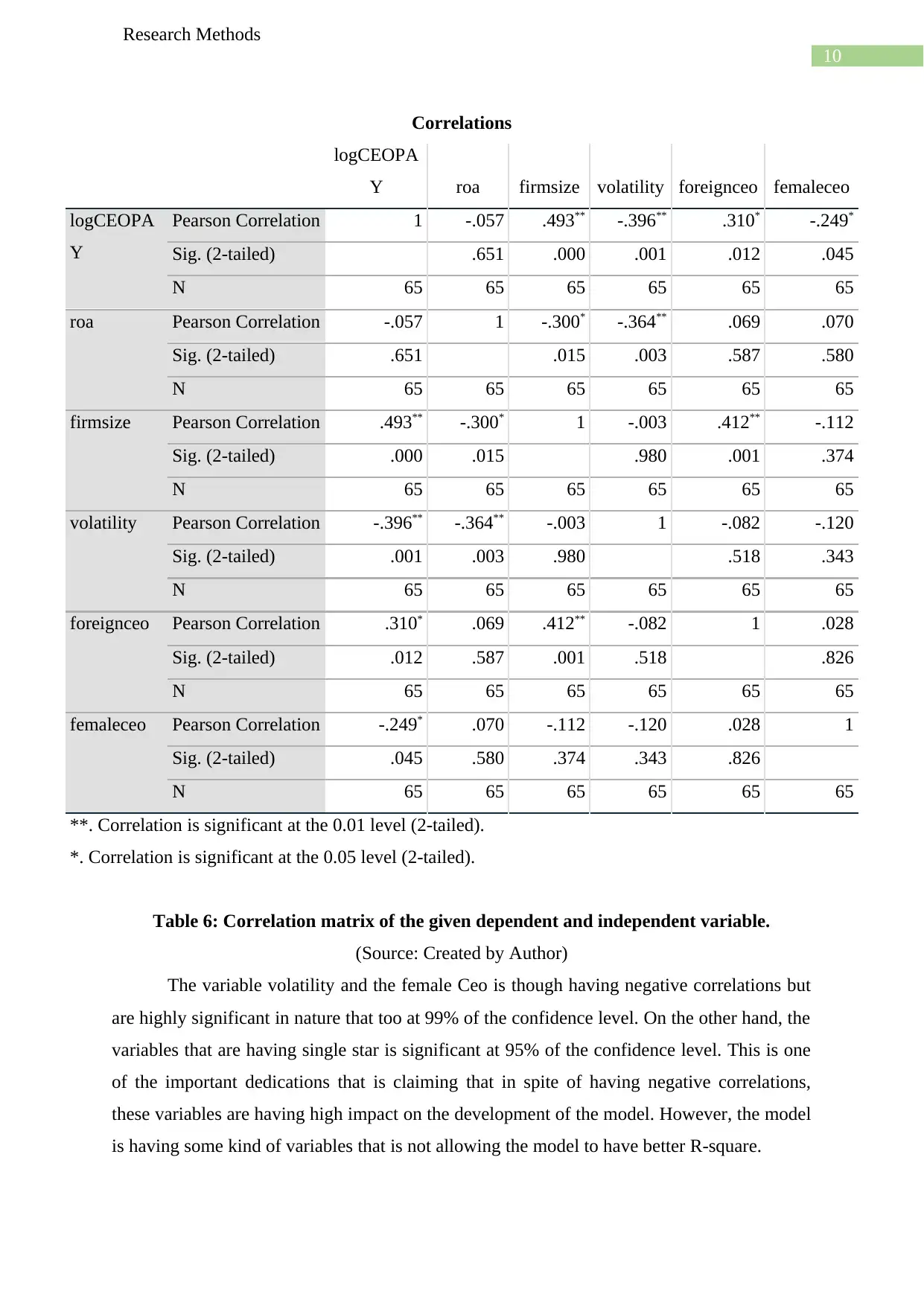
Table 6: Correlation matrix of the given dependent and independent variable.
(Source: Created by Author)
The variable volatility and the female Ceo is though having negative correlations but
are highly significant in nature that too at 99% of the confidence level. On the other hand, the
variables that are having single star is significant at 95% of the confidence level. This is one
of the important dedications that is claiming that in spite of having negative correlations,
these variables are having high impact on the development of the model. However, the model
is having some kind of variables that is not allowing the model to have better R-square.

11
Research Methods
3. Discussion of findings relating with relevant literature
Carroll (2017) opined that in order to determine the development of the model, it is
important to consider the variable at first that are going to have significant impact on the
mode. It has been opined that making the regression model effective in nature will definitely
bring in effective innovations. Through the development of better regression model, it is
important to indulge better techniques of sample collection that will increase the probability
of having better R-squared and adjusted R-squared. Through the development of this
regression analysis, it will be possible for the statistical analysis to introduce better model
development.
According to Chatterjee and Hadi (2015), the development of the regression analysis
will take on the development of variables that will not only lie within the significant values
but will also increase the development of the authenticity of the model. The regression
analysis will not only induce the development of the eternal strength and will highlight the
dependence of the independent variables on the dependent variable. On the other hand, it is
important to integrate variables in the model having the identification that will increase the
model verification. Through the identification of the variables it is important to increase the
resource of the modelling of data.
As opined by Darlington and Hayes (2016), in order to find the regression analysis
and linear model is helpful for the development of correlation coefficient is important in the
sense that through the development of the correlation coefficient it is important for the
statisticians to indulge the development of the business by predicting the variable.
4. Optional Opportunity for Individual Initiative
In order to discuss about the CEO compensations, it is important to include some of
the important variables in the sense that through the development of better model, it is
important to introduce the benefits that the most of the CEO will be taking as part of the
individual initiative that will help in the development of the return through the development
of the business. In order to increase the model development of ceo salary, it is important to
undertake certain variables that will not only increase the development of the model but will
also indulge the development of ceo salary. Through the development of better innovation
technologies. Through the development of the model, it is important for the involvement of

12
Research Methods
better introduction of regression that will not only increase the resources utilisation but will
also indulge the formation of the modules taking the variables that will be indulging the
development of variables like education of the CEO, working experience of the CEO, the
working technologies that has been invented by the CEO. Through the development of the
business, the company is indulging the development of business and these variables will
definitely improve the models so that the development of the regression become easy that
will be able to define the development of better innovations.
Part II: Tests for Weak Form Efficiency
Descriptive Statistics
N
Rang
e
Minim
um
Maxim
um Sum Mean
Std.
Deviat
ion
Varia
nce Skewness Kurtosis
Statis
tic
Statis
tic
Statisti
c
Statisti
c
Statis
tic
Statis
tic
Statisti
c
Statist
ic
Statis
tic
Std
.
Err
or
Statis
tic
Std
.
Err
or
Rt 501 10.76 -5.29 5.46 9.75 .0195 1.1516
1
1.326 -.225 .10
9
3.326 .21
8
Valid
N
(listwi
se)
501
Table 7: Summary Statistics for the Rt variable
(Source: Created by Author)
𝑅𝑡 = 𝑌𝑡 − 𝑌𝑡−1/ 𝑌𝑡−1 × 100 is the required formula that is being used for the
development of the Rt variable. The Rt variable is showing the return of the investment. Yt is
the adjusted closing stock price at the time period of t and Yt_1 is the adjusted closing stock
price in the time period of t_1. Through the development of this kind of model, it is possible
to know the return and will be able to predict the future consequences of the time series
model. Time series is also a part of the linear regression that takes the time into consideration.

13
Research Methods
Through the development of the time series the determination of the lag variable is possible
to calculate so that the seasonal adjustments can be easily made.
Step 2: Tests of Weak Form Efficiency
1) Descriptive Statistics and return distributions
Descriptive Statistics
N
Rang
e
Minim
um
Maxim
um Sum Mean
Std.
Deviat
ion
Varia
nce Skewness Kurtosis
Statis
tic
Statis
tic
Statisti
c
Statisti
c
Statis
tic
Statis
tic
Statisti
c
Statist
ic
Statis
tic
Std
.
Err
or
Statis
tic
Std
.
Err
or
Rt_1 500 10.76 -5.29 5.46 7.56 .0151 1.1486
5
1.319 -.229 .10
9
3.376 .21
8
Rt 501 10.76 -5.29 5.46 9.75 .0195 1.1516
1
1.326 -.225 .10
9
3.326 .21
8
Valid
N
(listwi
se)
500
Table 7: Summary Statistics for the Rt and Rt_1 variable
(Source: Created by Author)
2) Autoregressive (AR) Model
Correlations
Rt Rt_1
Pearson
Correlation
Rt 1.000 -.070
Rt_1 -.070 1.000
Sig. (1-tailed) Rt . .060

14
Research Methods
Rt_1 .060 .
N Rt 500 500
Rt_1 500 500
Model Summaryb
Model R
R
Square
Adjusted
R Square
Std. Error
of the
Estimate
Change Statistics
Durbin-
Watson
R
Square
Change
F
Change df1 df2
Sig. F
Change
1 .070a .005 .003 1.14974 .005 2.422 1 498 .120 2.000
a. Predictors: (Constant), Rt_1
b. Dependent Variable: Rt
ANOVAa
Model
Sum of
Squares df Mean Square F Sig.
1 Regression 3.202 1 3.202 2.422 .120b
Residual 658.306 498 1.322
Total 661.508 499
a. Dependent Variable: Rt
b. Predictors: (Constant), Rt_1
Coefficientsa
Model
Unstandardized
Coefficients
Standardized
Coefficients
t Sig.
95.0% Confidence
Interval for B
B Std. Error Beta
Lower
Bound
Upper
Bound
1 (Constant
)
.018 .051 .350 .727 -.083 .119
Rt_1 -.070 .045 -.070 -
1.556
.120 -.158 .018

15
Research Methods
a. Dependent Variable: Rt
In the above figure, the 𝑅𝑡=𝛼+𝛽𝑅𝑡−1+𝜀𝑡 and putting the values from the above table, it
can be claimed that the 𝑅𝑡=0.018-0.070 𝑅𝑡−1. There existing negative correlation among
these two variables.
Walt Disney
Descriptive Statistics
Mean
Std.
Deviation N
Rt .0169 1.15138 500
Rt_1 .0151 1.14865 500
Correlations
Rt Rt_1
Pearson
Correlation
Rt 1.000 -.070
Rt_1 -.070 1.000
Sig. (1-tailed) Rt . .060
Rt_1 .060 .
N Rt 500 500
Rt_1 500 500
Model Summaryb
Model R
R
Square
Adjusted
R Square
Std. Error
of the
Estimate
Change Statistics
Durbin-
Watson
R
Square
Change
F
Change df1 df2
Sig. F
Change
1 .070a .005 .003 1.14974 .005 2.422 1 498 .120 2.000
a. Predictors: (Constant), Rt_1
b. Dependent Variable: Rt

16
Research Methods

17
Research Methods
ANOVAa
Model
Sum of
Squares df Mean Square F Sig.
1 Regression 3.202 1 3.202 2.422 .120b
Residual 658.306 498 1.322
Total 661.508 499
a. Dependent Variable: Rt
b. Predictors: (Constant), Rt_1
Coefficientsa
Model
Unstandardized
Coefficients
Standardized
Coefficients
t Sig.
99.0%
Confidence
Interval for B
Collinearity
Statistics
B
Std.
Error Beta
Lower
Bound
Upper
Bound Tolerance VIF
1 (Constant
)
.018 .051 .350 .727 -.115 .151
Rt_1 -.070 .045 -.070 -
1.556
.120 -.186 .046 1.000 1.000
a. Dependent Variable: Rt
In the above figure, the 𝑅𝑡=𝛼+𝛽𝑅𝑡−1+𝜀𝑡 and putting the values from the above table, it
can be claimed that the 𝑅𝑡=0.018-0.070 𝑅𝑡−1. There existing negative correlation among
these two variables.
Conclusion
The wholes study has seen the development of statistics, using two companies Walt
Disney and 21st Century Fox. The study has defined the development of the ARIMA model
and the linear model taking the lag variable. On the other hand, the development of better
technologies will bring in involvement of better designs that will definitely increase the
development of better policy formation. The whole study is important in showing the
relationship among the daily stock prices of two companies. Various linear regressions has
been done and empirical results has been calculated.

18
Research Methods
Reference list
Carroll, R.J., 2017. Transformation and weighting in regression. Routledge.
Chatterjee, S. and Hadi, A.S., 2015. Regression analysis by example. John Wiley & Sons.
Darlington, R.B. and Hayes, A.F., 2016. Regression analysis and linear models: Concepts,
applications, and implementation. Guilford Publications.
Dimos, C. and Pugh, G., 2016. The effectiveness of R&D subsidies: A meta-regression
analysis of the evaluation literature. Research Policy, 45(4), pp.797-815.
Fox, J., 2015. Applied regression analysis and generalized linear models. Sage Publications.
Galling, B., Roldan, A., Hagi, K., Rietschel, L., Walyzada, F., Zheng, W., Cao, X.L., Xiang,
Y.T., Zink, M., Kane, J.M. and Nielsen, J., 2017. Antipsychotic augmentation vs.
monotherapy in schizophrenia: systematic review, meta‐analysis and meta‐regression
analysis. World Psychiatry, 16(1), pp.77-89.
Gechert, S., 2015. What fiscal policy is most effective? A meta-regression analysis. Oxford
Economic Papers, 67(3), pp.553-580.
Harrell Jr, F.E., 2015. Regression modeling strategies: with applications to linear models,
logistic and ordinal regression, and survival analysis. Springer.
Hayes, A.F., 2017. Introduction to mediation, moderation, and conditional process analysis:
A regression-based approach. Guilford Publications.
Hui, F.K., 2016. boral–Bayesian ordination and regression analysis of multivariate abundance
data in R. Methods in Ecology and Evolution, 7(6), pp.744-750.
Levine, H., Jørgensen, N., Martino-Andrade, A., Mendiola, J., Weksler-Derri, D., Mindlis, I.,
Pinotti, R. and Swan, S.H., 2017. Temporal trends in sperm count: a systematic review and
meta-regression analysis. Human reproduction update, 23(6), pp.646-659.
Onrust, S.A., Otten, R., Lammers, J. and Smit, F., 2016. School-based programmes to reduce
and prevent substance use in different age groups: What works for whom? Systematic review
and meta-regression analysis. Clinical Psychology Review, 44, pp.45-59.
Silverman, B.W., 2018. Density estimation for statistics and data analysis. Routledge.