In-depth Homework: Statistical Data Analysis, Interpretation & Results
VerifiedAdded on 2023/06/18
|40
|5876
|414
Homework Assignment
AI Summary
This assignment solution covers a range of statistical analyses performed on various datasets. Week 1 focuses on descriptive statistics, including mean attitudinal scores and boxplot interpretations for Republican and Democrat respondents. Week 2 involves computing skewness, kurtosis, mean, and standard deviation for anxiety scores, with interpretations on normality and data spread. Week 3 includes frequency analysis on gender, marital status, and education levels, along with percentile rank calculations for anxiety scores under normal and non-normal distribution assumptions. Week 4 provides analysis of eating time data using t-tests and homogeneity of variance tests. Week 5 involves one-way ANOVA and post-hoc tests, and examines the relationship between hair color and extrovertedness. Week 6 focuses on linear regression, exploring the relationship between multiple R and bivariate correlation. Finally, Week 7 covers multiple regression analysis and factor analysis on SCVS data, identifying underlying factors based on scree plots and eigenvalue criteria. The document provides detailed results and interpretations for each statistical test performed.

1
RESEARCH QUESTIONS
RESEARCH QUESTIONS
Paraphrase This Document
Need a fresh take? Get an instant paraphrase of this document with our AI Paraphraser
2
Table of Contents
WEEK 1...........................................................................................................................................4
WEEK 2...........................................................................................................................................9
WEEK 3.........................................................................................................................................10
WEEK 4- Lesson 24 Exercise File 1.............................................................................................19
Results for the test evaluating homogeneity of variance...........................................................19
3. Cohen’s d effect.....................................................................................................................21
5. Boxplot..................................................................................................................................22
Week 4 - Lesson 41 Exercise File 1..............................................................................................22
a, b & c.......................................................................................................................................22
d)................................................................................................................................................23
2. Clustered graph......................................................................................................................24
3. Results....................................................................................................................................24
WEEK-5........................................................................................................................................25
1. One way annova and post hoc test.........................................................................................25
2. Relationship between hair colour and extrovertedness.........................................................27
3. Boxplot..................................................................................................................................27
WEEK-6........................................................................................................................................28
Linear regression.......................................................................................................................28
Relationship between multiple R and bivariate correlation.......................................................31
Scatterplot..................................................................................................................................31
Result section.............................................................................................................................32
WEEK-7........................................................................................................................................32
Regression..................................................................................................................................32
1. Multiple regression................................................................................................................32
2. Regression equation...............................................................................................................32
3. and 4. Performance of the regression analysis.......................................................................33
Factor analysis...........................................................................................................................36
1. Factors underlying in SCVS on the basis of scree plot.........................................................38

3
2. Factor based on eigenvalue greater than 1 criterion..............................................................39
3. Result section.........................................................................................................................39
REFERENCES................................................................................................................................1
⊘ This is a preview!⊘
Do you want full access?
Subscribe today to unlock all pages.
Trusted by 1+ million students worldwide

4
WEEK 1
Lesson 21, Exercise File 2
Mean Attitudinal scores:
For Republican respondents:
Descriptive Statistics
N Minimum Maximum Sum Mean
att1 21 1 5 68 3.24
att2 21 2 4 69 3.29
att3 21 2 5 73 3.48
att4 21 2 5 70 3.33
att5 21 1 4 49 2.33
Valid N (listwise) 21
Interpretation:
From the above table it has been found that the mean of att1 is 3.24, att2 is 3.29, att3 is 3.48,
att4 is 3.33 and att5 is 2.33. Thus it can be interpreted that on an average, respondents had
neutral views for att1, att2, att3, att4 while for att5, average number of respondents disagreed.
For Democrat respondents:
Descriptive Statistics
N Minimum Maximum Sum Mean
att1 19 1 4 53 2.79
att2 19 1 4 44 2.32
att3 19 1 3 41 2.16
att4 19 1 3 39 2.05
Paraphrase This Document
Need a fresh take? Get an instant paraphrase of this document with our AI Paraphraser
5
att5 19 1 4 33 1.74
Valid N (listwise) 19
Interpretation:
From the above table it can be understood that the mean of att1 is 2.79, att2 is 2.32, att3 is
2.16, att4 is 2.05 and att5 is 1.74. Hence, it can be interpreted that the average number of
respondents have disagree view for att1, att2, att3, att4. However, for att5 the view is highly
disagree.
Total attitude scores from the scores for the five attitudinal items:
The total attitude score of Republic party is 329 while that of Democrat party is 210.
Means on the total attitude scores for the two political parties:
The mean of Republic party is 15.66 while that of Democrat party is 11.05.
Boxplot:
For Republic party:
Case Processing Summary
Cases
Valid Missing Total
N Percent N Percent N Percent

6
att1 21 100.0% 0 0.0% 21 100.0%
att2 21 100.0% 0 0.0% 21 100.0%
att3 21 100.0% 0 0.0% 21 100.0%
att4 21 100.0% 0 0.0% 21 100.0%
att5 21 100.0% 0 0.0% 21 100.0%
Interpretation:
From the above boxplot it can be interpreted that tall boxplots for att1, att3 and att5 show
that different attitudes are held by students in republican party. Also, there is a striking difference
between the responses for att5 as compared to the other attitudes.
⊘ This is a preview!⊘
Do you want full access?
Subscribe today to unlock all pages.
Trusted by 1+ million students worldwide
7
For Democrat party:
Case Processing Summary
Cases
Valid Missing Total
N Percent N Percent N Percent
att1 19 100.0% 0 0.0% 19 100.0%
att2 19 100.0% 0 0.0% 19 100.0%
att3 19 100.0% 0 0.0% 19 100.0%
att4 19 100.0% 0 0.0% 19 100.0%
att5 19 100.0% 0 0.0% 19 100.0%
For Democrat party:
Case Processing Summary
Cases
Valid Missing Total
N Percent N Percent N Percent
att1 19 100.0% 0 0.0% 19 100.0%
att2 19 100.0% 0 0.0% 19 100.0%
att3 19 100.0% 0 0.0% 19 100.0%
att4 19 100.0% 0 0.0% 19 100.0%
att5 19 100.0% 0 0.0% 19 100.0%
Paraphrase This Document
Need a fresh take? Get an instant paraphrase of this document with our AI Paraphraser
8
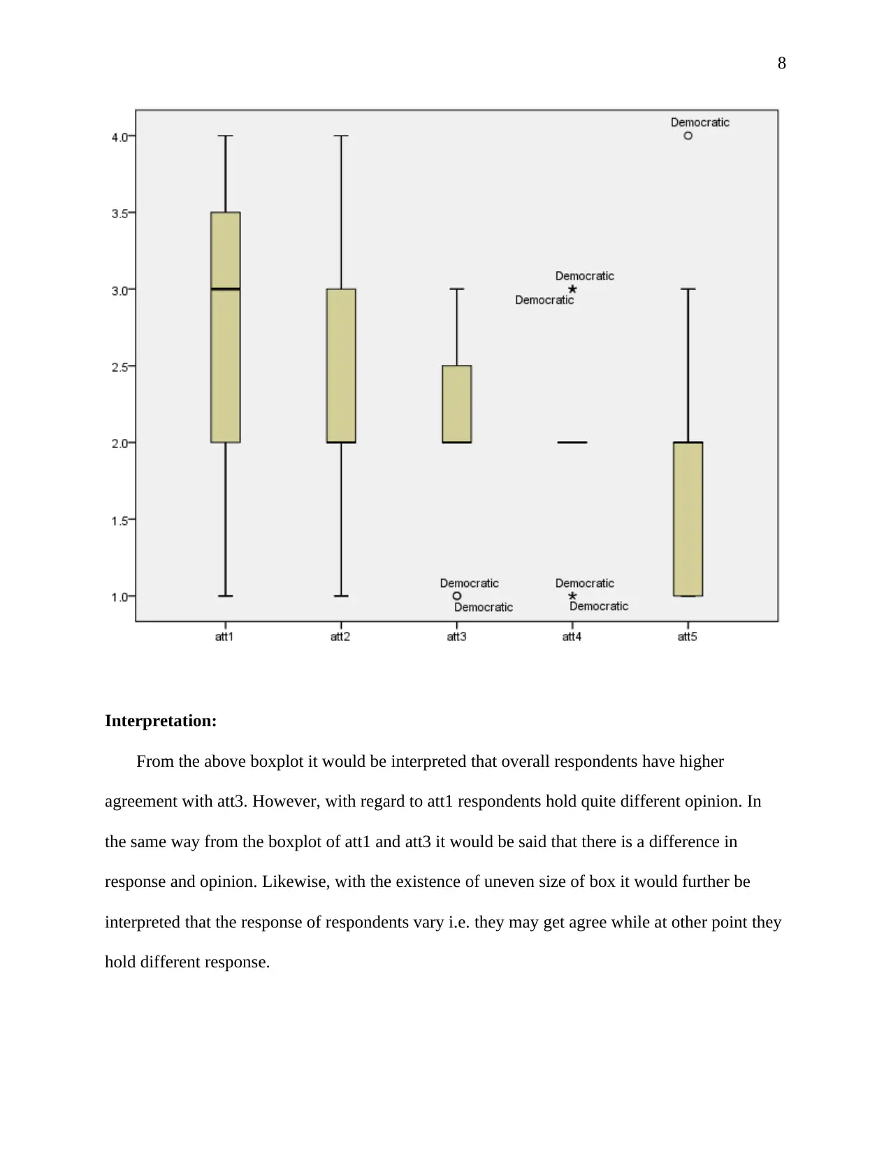
Interpretation:
From the above boxplot it would be interpreted that overall respondents have higher
agreement with att3. However, with regard to att1 respondents hold quite different opinion. In
the same way from the boxplot of att1 and att3 it would be said that there is a difference in
response and opinion. Likewise, with the existence of uneven size of box it would further be
interpreted that the response of respondents vary i.e. they may get agree while at other point they
hold different response.

9
WEEK 2
Lesson 21 Exercise File 1
Computation of Skewness, Mean, Standard Deviation, and Kurtosis of anxiety scores:
Descriptive Statistics
N Minimum Maximum Mean Std.
Deviation
Skewness Kurtosis
Statistic Statistic Statistic Statistic Statistic Statistic Std. Error Statistic Std. Error
Anxiety Scores 15 5 78 32.27 23.478 .416 .580 -1.124 1.121
Valid N
(listwise)
15
Result section:
As the ideal range of Skewness and Kurtosis for measuring its distribution is ± 1.0 (Hair
Jr, and et.al., 2021). And as per the above calculation it would be analyzed that the Skewness of
the respondent’s anxiety is 0.416 which is falling in the category of ± 1.0. This means it would
be right to interpreted that the respondent’s anxiety scores fall in the category of normality, i.e.
the distribution lies in normal category. However, while analysing the Kurtosis, it can be
observed that the value of Kurtosis is -1.124 which is certainly lower than the ideal range of ±
1.0. Thus, it can be interpreted that the distribution of Kurtosis is too flat.
In the same from the above table it is also observed that the mean of anxiety score is
32.27 while the standard deviation is 23.478 (Green, Salkind, 2017). Thus, it can be interpreted
that the standard deviation of the dataset i.e. respondent’s anxiety is high because the data point
is spread at a large range.
⊘ This is a preview!⊘
Do you want full access?
Subscribe today to unlock all pages.
Trusted by 1+ million students worldwide

10
In the same it can also be interpreted that as the mean of students is 32.27 which depict that
the average number of students suffers from severe anxiety. This is because as per the range of
anxiety the score of 30-63 shows the anxiety of severe extent.
WEEK 3
Exercise 1 Lesson 20
Frequency analysis on the gender and marital status:
Percentage of men
Gender
Frequency Percent Valid Percent Cumulative Percent
Valid
Men 13 52.0 52.0 52.0
Women 12 48.0 48.0 100.0
Total 25 100.0 100.0
Results:
From the above table it can be evaluated that there is an unequal percent breakout. As
there are 52% are men while that of 48% are women. This mean that the percent of men are more
in comparison with women.
Mode of marital status
Statistics
Marital Status
N Valid 25
Paraphrase This Document
Need a fresh take? Get an instant paraphrase of this document with our AI Paraphraser

11
Missing 0
Mode 2
Interpretation:
From the above table it can be analyzed that the mode of marital status is 2 which means
that majority are carrying a status of Divorced.
Frequency of divorced people
Marital Status
Frequency Percent Valid Percent Cumulative Percent
Valid
Married 9 36.0 36.0 36.0
Divorced 11 44.0 44.0 80.0
Never Married 5 20.0 20.0 100.0
Total 25 100.0 100.0
Interpretation:
As per the above table it can be evaluated that the frequency of Divorced are 11 which is the
highest. This means that there is a majority of respondent who are Divorced.
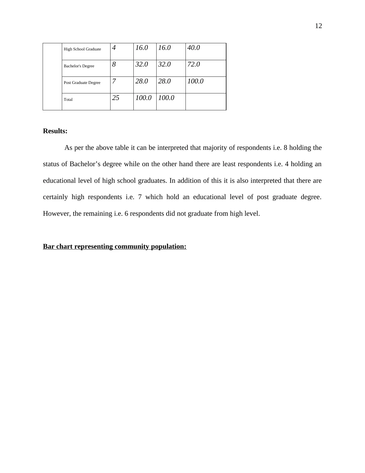
Frequency table of educational level of respondents:
Education Level
Frequency Percent Valid Percent Cumulative Percent
Valid Did not graduate from
high school
6 24.0 24.0 24.0
Missing 0
Mode 2
Interpretation:
From the above table it can be analyzed that the mode of marital status is 2 which means
that majority are carrying a status of Divorced.
Frequency of divorced people
Marital Status
Frequency Percent Valid Percent Cumulative Percent
Valid
Married 9 36.0 36.0 36.0
Divorced 11 44.0 44.0 80.0
Never Married 5 20.0 20.0 100.0
Total 25 100.0 100.0
Interpretation:
As per the above table it can be evaluated that the frequency of Divorced are 11 which is the
highest. This means that there is a majority of respondent who are Divorced.
Frequency table of educational level of respondents:
Education Level
Frequency Percent Valid Percent Cumulative Percent
Valid Did not graduate from
high school
6 24.0 24.0 24.0
12
High School Graduate 4 16.0 16.0 40.0
Bachelor's Degree 8 32.0 32.0 72.0
Post Graduate Degree 7 28.0 28.0 100.0
Total 25 100.0 100.0
Results:
As per the above table it can be interpreted that majority of respondents i.e. 8 holding the
status of Bachelor’s degree while on the other hand there are least respondents i.e. 4 holding an
educational level of high school graduates. In addition of this it is also interpreted that there are
certainly high respondents i.e. 7 which hold an educational level of post graduate degree.
However, the remaining i.e. 6 respondents did not graduate from high level.
Bar chart representing community population:
⊘ This is a preview!⊘
Do you want full access?
Subscribe today to unlock all pages.
Trusted by 1+ million students worldwide
1 out of 40
Your All-in-One AI-Powered Toolkit for Academic Success.
+13062052269
info@desklib.com
Available 24*7 on WhatsApp / Email
![[object Object]](/_next/static/media/star-bottom.7253800d.svg)
Unlock your academic potential
Copyright © 2020–2025 A2Z Services. All Rights Reserved. Developed and managed by ZUCOL.