Statistics for Business: Stock Analysis, Hypothesis Testing and CAPM

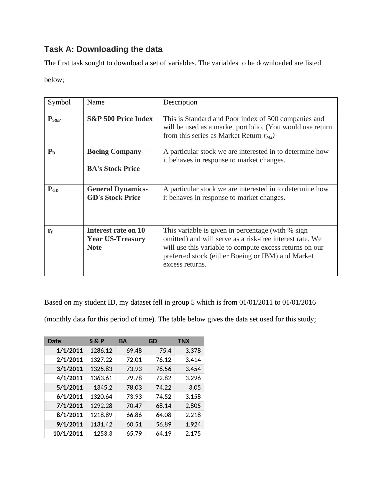
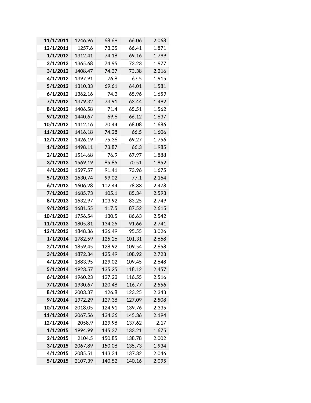
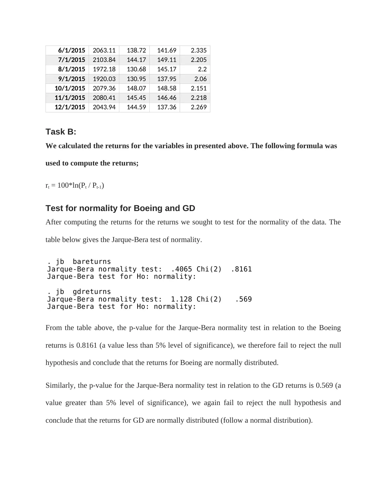
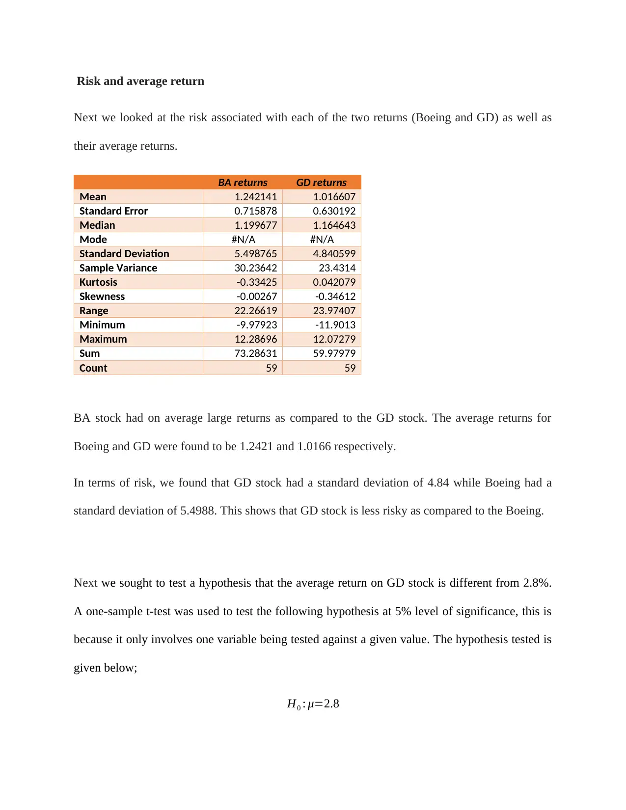
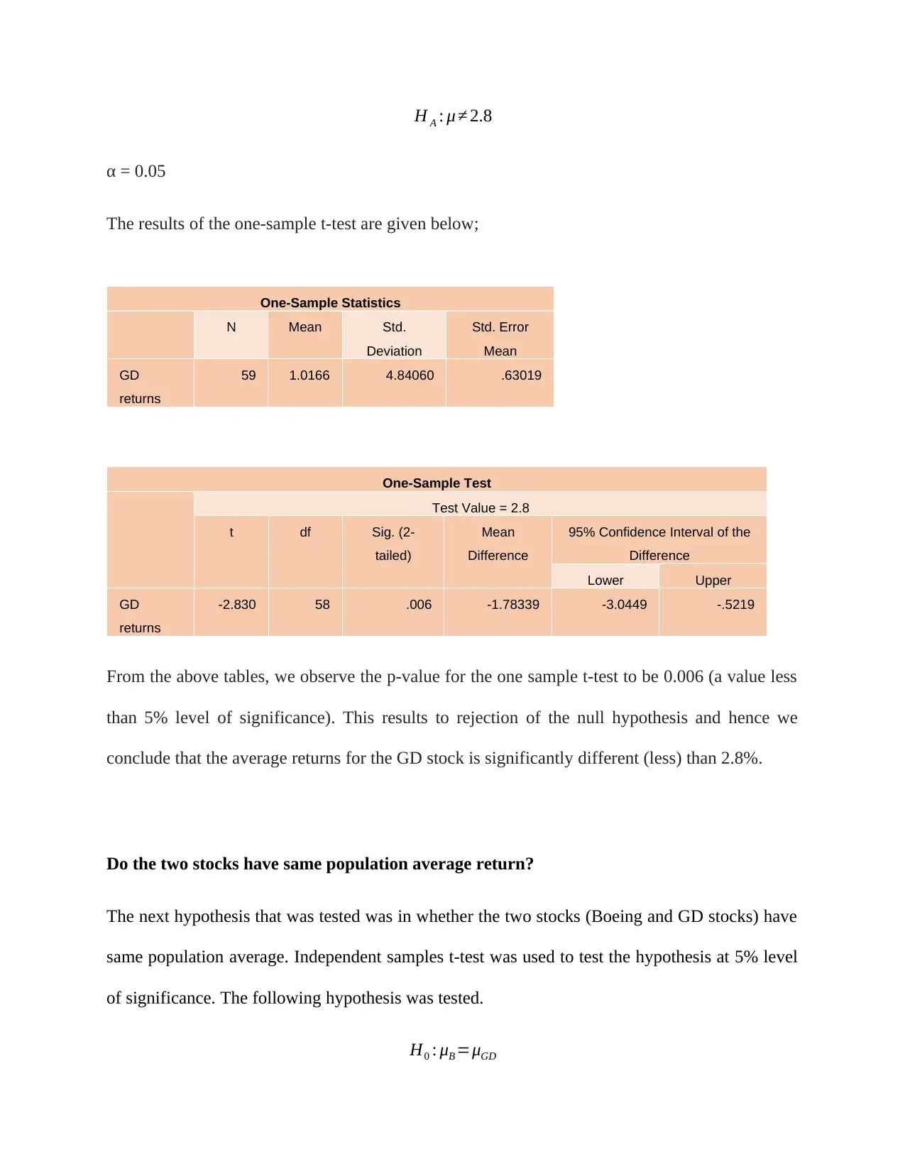
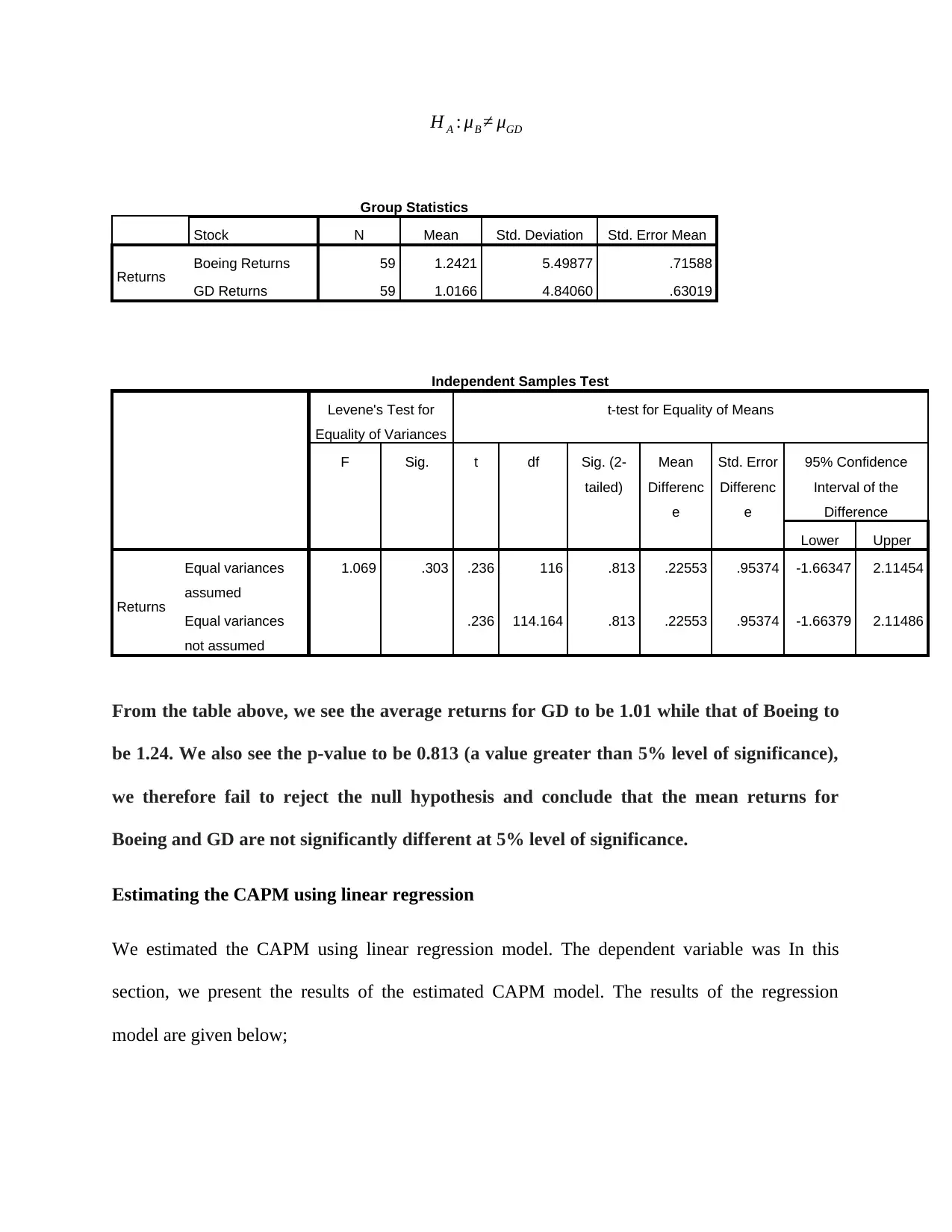
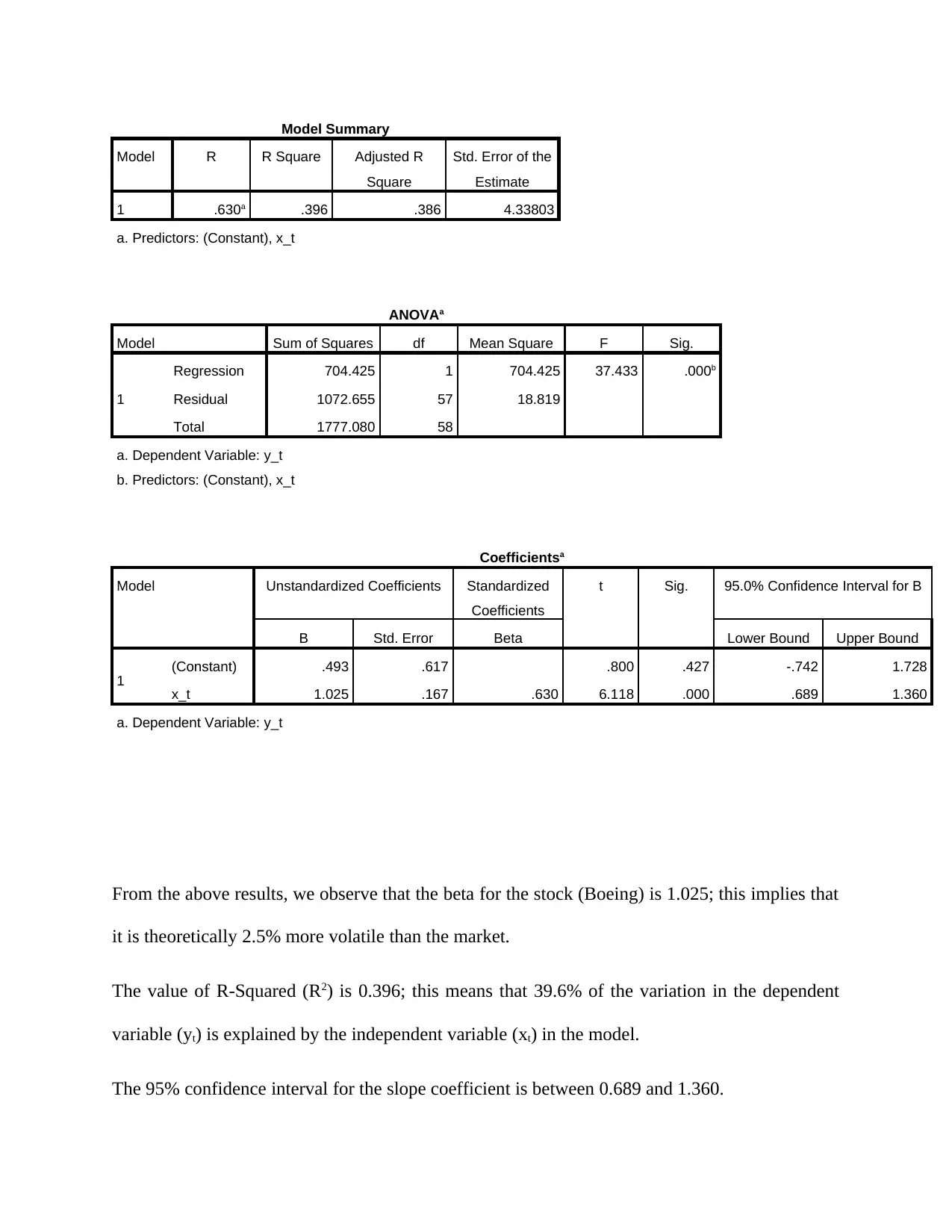
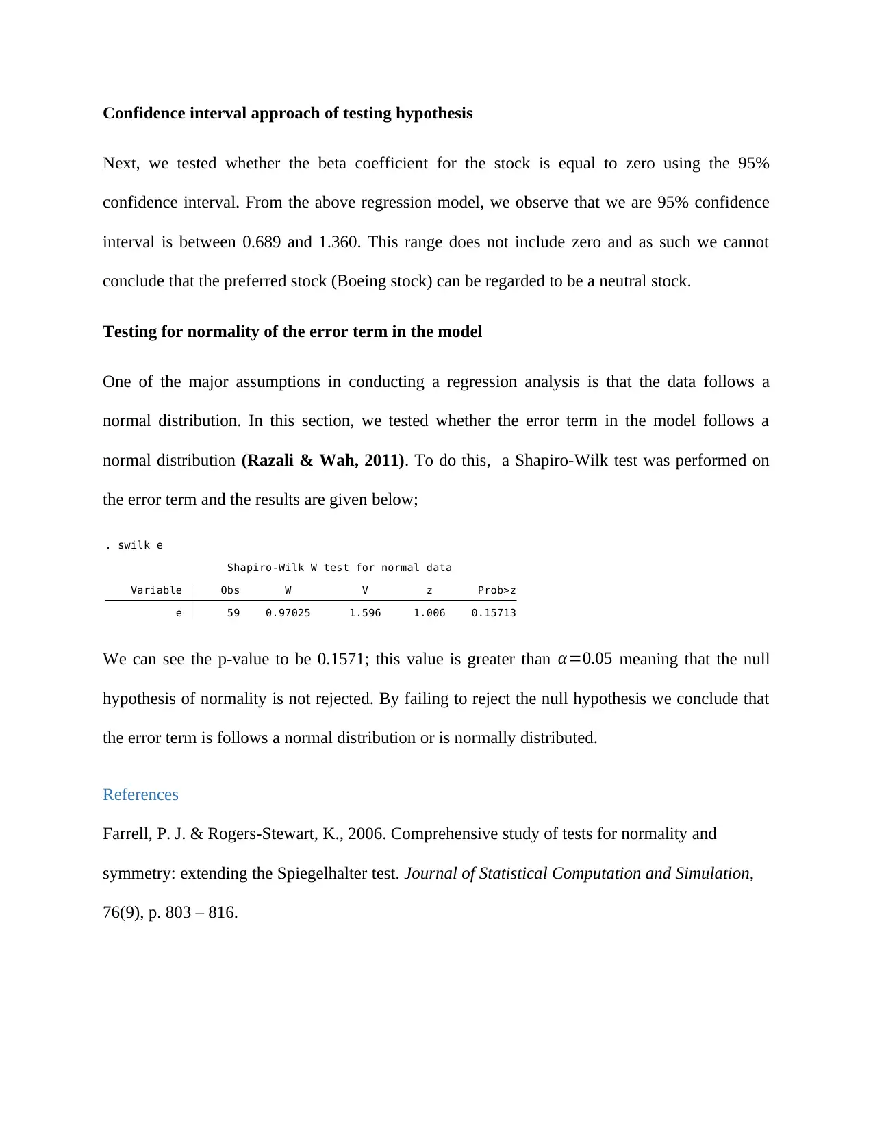
This report provides a statistical analysis of stock returns for Boeing (BA) and General Dynamics (GD), utilizing data from January 2011 to January 2016. The analysis includes calculating returns, testing for normality using the Jarque-Bera test, and comparing the risk and average returns of both stocks. Hypothesis testing is conducted to determine if the average return on GD stock differs from 2.8% and whether the two stocks have the same population average return, employing one-sample and independent samples t-tests, respectively. Furthermore, the Capital Asset Pricing Model (CAPM) is estimated using linear regression, and the beta coefficient for Boeing is analyzed. The normality of the error term in the regression model is assessed using the Shapiro-Wilk test. The report concludes with interpretations of the statistical results and their implications for investment decisions.

Statistics for business
Name:
Institution:
30th May 2018

Task A: Downloading the data
The first task sought to download a set of variables. The variables to be downloaded are listed
below;
Symbol Name Description
PS&P S&P 500 Price Index This is Standard and Poor index of 500 companies and
will be used as a market portfolio. (You would use return
from this series as Market Return rM,t)
PB Boeing Company-
BA's Stock Price
A particular stock we are interested in to determine how
it behaves in response to market changes.
PGD General Dynamics-
GD's Stock Price
A particular stock we are interested in to determine how
it behaves in response to market changes.
rf Interest rate on 10
Year US-Treasury
Note
This variable is given in percentage (with % sign
omitted) and will serve as a risk-free interest rate. We
will use this variable to compute excess returns on our
preferred stock (either Boeing or IBM) and Market
excess returns.
Based on my student ID, my dataset fell in group 5 which is from 01/01/2011 to 01/01/2016
(monthly data for this period of time). The table below gives the data set used for this study;
Date S & P BA GD TNX
1/1/2011 1286.12 69.48 75.4 3.378
2/1/2011 1327.22 72.01 76.12 3.414
3/1/2011 1325.83 73.93 76.56 3.454
4/1/2011 1363.61 79.78 72.82 3.296
5/1/2011 1345.2 78.03 74.22 3.05
6/1/2011 1320.64 73.93 74.52 3.158
7/1/2011 1292.28 70.47 68.14 2.805
8/1/2011 1218.89 66.86 64.08 2.218
9/1/2011 1131.42 60.51 56.89 1.924
10/1/2011 1253.3 65.79 64.19 2.175

11/1/2011 1246.96 68.69 66.06 2.068
12/1/2011 1257.6 73.35 66.41 1.871
1/1/2012 1312.41 74.18 69.16 1.799
2/1/2012 1365.68 74.95 73.23 1.977
3/1/2012 1408.47 74.37 73.38 2.216
4/1/2012 1397.91 76.8 67.5 1.915
5/1/2012 1310.33 69.61 64.01 1.581
6/1/2012 1362.16 74.3 65.96 1.659
7/1/2012 1379.32 73.91 63.44 1.492
8/1/2012 1406.58 71.4 65.51 1.562
9/1/2012 1440.67 69.6 66.12 1.637
10/1/2012 1412.16 70.44 68.08 1.686
11/1/2012 1416.18 74.28 66.5 1.606
12/1/2012 1426.19 75.36 69.27 1.756
1/1/2013 1498.11 73.87 66.3 1.985
2/1/2013 1514.68 76.9 67.97 1.888
3/1/2013 1569.19 85.85 70.51 1.852
4/1/2013 1597.57 91.41 73.96 1.675
5/1/2013 1630.74 99.02 77.1 2.164
6/1/2013 1606.28 102.44 78.33 2.478
7/1/2013 1685.73 105.1 85.34 2.593
8/1/2013 1632.97 103.92 83.25 2.749
9/1/2013 1681.55 117.5 87.52 2.615
10/1/2013 1756.54 130.5 86.63 2.542
11/1/2013 1805.81 134.25 91.66 2.741
12/1/2013 1848.36 136.49 95.55 3.026
1/1/2014 1782.59 125.26 101.31 2.668
2/1/2014 1859.45 128.92 109.54 2.658
3/1/2014 1872.34 125.49 108.92 2.723
4/1/2014 1883.95 129.02 109.45 2.648
5/1/2014 1923.57 135.25 118.12 2.457
6/1/2014 1960.23 127.23 116.55 2.516
7/1/2014 1930.67 120.48 116.77 2.556
8/1/2014 2003.37 126.8 123.25 2.343
9/1/2014 1972.29 127.38 127.09 2.508
10/1/2014 2018.05 124.91 139.76 2.335
11/1/2014 2067.56 134.36 145.36 2.194
12/1/2014 2058.9 129.98 137.62 2.17
1/1/2015 1994.99 145.37 133.21 1.675
2/1/2015 2104.5 150.85 138.78 2.002
3/1/2015 2067.89 150.08 135.73 1.934
4/1/2015 2085.51 143.34 137.32 2.046
5/1/2015 2107.39 140.52 140.16 2.095

6/1/2015 2063.11 138.72 141.69 2.335
7/1/2015 2103.84 144.17 149.11 2.205
8/1/2015 1972.18 130.68 145.17 2.2
9/1/2015 1920.03 130.95 137.95 2.06
10/1/2015 2079.36 148.07 148.58 2.151
11/1/2015 2080.41 145.45 146.46 2.218
12/1/2015 2043.94 144.59 137.36 2.269
Task B:
We calculated the returns for the variables in presented above. The following formula was
used to compute the returns;
rt = 100*ln(Pt / Pt-1)
Test for normality for Boeing and GD
After computing the returns for the returns we sought to test for the normality of the data. The
table below gives the Jarque-Bera test of normality.
Jarque-Bera test for Ho: normality:
Jarque-Bera normality test: 1.128 Chi(2) .569
. jb gdreturns
Jarque-Bera test for Ho: normality:
Jarque-Bera normality test: .4065 Chi(2) .8161
. jb bareturns
From the table above, the p-value for the Jarque-Bera normality test in relation to the Boeing
returns is 0.8161 (a value less than 5% level of significance), we therefore fail to reject the null
hypothesis and conclude that the returns for Boeing are normally distributed.
Similarly, the p-value for the Jarque-Bera normality test in relation to the GD returns is 0.569 (a
value greater than 5% level of significance), we again fail to reject the null hypothesis and
conclude that the returns for GD are normally distributed (follow a normal distribution).

Risk and average return
Next we looked at the risk associated with each of the two returns (Boeing and GD) as well as
their average returns.
BA returns GD returns
Mean 1.242141 1.016607
Standard Error 0.715878 0.630192
Median 1.199677 1.164643
Mode #N/A #N/A
Standard Deviation 5.498765 4.840599
Sample Variance 30.23642 23.4314
Kurtosis -0.33425 0.042079
Skewness -0.00267 -0.34612
Range 22.26619 23.97407
Minimum -9.97923 -11.9013
Maximum 12.28696 12.07279
Sum 73.28631 59.97979
Count 59 59
BA stock had on average large returns as compared to the GD stock. The average returns for
Boeing and GD were found to be 1.2421 and 1.0166 respectively.
In terms of risk, we found that GD stock had a standard deviation of 4.84 while Boeing had a
standard deviation of 5.4988. This shows that GD stock is less risky as compared to the Boeing.
Next we sought to test a hypothesis that the average return on GD stock is different from 2.8%.
A one-sample t-test was used to test the following hypothesis at 5% level of significance, this is
because it only involves one variable being tested against a given value. The hypothesis tested is
given below;
H0 : μ=2.8

H A : μ ≠ 2.8
α = 0.05
The results of the one-sample t-test are given below;
One-Sample Statistics
N Mean Std.
Deviation
Std. Error
Mean
GD
returns
59 1.0166 4.84060 .63019
One-Sample Test
Test Value = 2.8
t df Sig. (2-
tailed)
Mean
Difference
95% Confidence Interval of the
Difference
Lower Upper
GD
returns
-2.830 58 .006 -1.78339 -3.0449 -.5219
From the above tables, we observe the p-value for the one sample t-test to be 0.006 (a value less
than 5% level of significance). This results to rejection of the null hypothesis and hence we
conclude that the average returns for the GD stock is significantly different (less) than 2.8%.
Do the two stocks have same population average return?
The next hypothesis that was tested was in whether the two stocks (Boeing and GD stocks) have
same population average. Independent samples t-test was used to test the hypothesis at 5% level
of significance. The following hypothesis was tested.
H0 : μB =μGD

H A : μB ≠ μGD
Group Statistics
Stock N Mean Std. Deviation Std. Error Mean
Returns Boeing Returns 59 1.2421 5.49877 .71588
GD Returns 59 1.0166 4.84060 .63019
Independent Samples Test
Levene's Test for
Equality of Variances
t-test for Equality of Means
F Sig. t df Sig. (2-
tailed)
Mean
Differenc
e
Std. Error
Differenc
e
95% Confidence
Interval of the
Difference
Lower Upper
Returns
Equal variances
assumed
1.069 .303 .236 116 .813 .22553 .95374 -1.66347 2.11454
Equal variances
not assumed
.236 114.164 .813 .22553 .95374 -1.66379 2.11486
From the table above, we see the average returns for GD to be 1.01 while that of Boeing to
be 1.24. We also see the p-value to be 0.813 (a value greater than 5% level of significance),
we therefore fail to reject the null hypothesis and conclude that the mean returns for
Boeing and GD are not significantly different at 5% level of significance.
Estimating the CAPM using linear regression
We estimated the CAPM using linear regression model. The dependent variable was In this
section, we present the results of the estimated CAPM model. The results of the regression
model are given below;

Model Summary
Model R R Square Adjusted R
Square
Std. Error of the
Estimate
1 .630a .396 .386 4.33803
a. Predictors: (Constant), x_t
ANOVAa
Model Sum of Squares df Mean Square F Sig.
1
Regression 704.425 1 704.425 37.433 .000b
Residual 1072.655 57 18.819
Total 1777.080 58
a. Dependent Variable: y_t
b. Predictors: (Constant), x_t
Coefficientsa
Model Unstandardized Coefficients Standardized
Coefficients
t Sig. 95.0% Confidence Interval for B
B Std. Error Beta Lower Bound Upper Bound
1 (Constant) .493 .617 .800 .427 -.742 1.728
x_t 1.025 .167 .630 6.118 .000 .689 1.360
a. Dependent Variable: y_t
From the above results, we observe that the beta for the stock (Boeing) is 1.025; this implies that
it is theoretically 2.5% more volatile than the market.
The value of R-Squared (R2) is 0.396; this means that 39.6% of the variation in the dependent
variable (yt) is explained by the independent variable (xt) in the model.
The 95% confidence interval for the slope coefficient is between 0.689 and 1.360.

Confidence interval approach of testing hypothesis
Next, we tested whether the beta coefficient for the stock is equal to zero using the 95%
confidence interval. From the above regression model, we observe that we are 95% confidence
interval is between 0.689 and 1.360. This range does not include zero and as such we cannot
conclude that the preferred stock (Boeing stock) can be regarded to be a neutral stock.
Testing for normality of the error term in the model
One of the major assumptions in conducting a regression analysis is that the data follows a
normal distribution. In this section, we tested whether the error term in the model follows a
normal distribution (Razali & Wah, 2011). To do this, a Shapiro-Wilk test was performed on
the error term and the results are given below;
e 59 0.97025 1.596 1.006 0.15713
Variable Obs W V z Prob>z
Shapiro-Wilk W test for normal data
. swilk e
We can see the p-value to be 0.1571; this value is greater than α =0.05 meaning that the null
hypothesis of normality is not rejected. By failing to reject the null hypothesis we conclude that
the error term is follows a normal distribution or is normally distributed.
References
Farrell, P. J. & Rogers-Stewart, K., 2006. Comprehensive study of tests for normality and
symmetry: extending the Spiegelhalter test. Journal of Statistical Computation and Simulation,
76(9), p. 803 – 816.

Razali, N. & Wah, Y. B., 2011. Power comparisons of Shapiro–Wilk, Kolmogorov–Smirnov,
Lilliefors and Anderson–Darling tests. Journal of Statistical Modeling and Analytics, 2(1), p. 21–
33.
Sawilowsky, S. S., 2005. Misconceptions Leading to Choosing the t Test Over The Wilcoxon
Mann–Whitney Test for Shift in Location Parameter. Journal of Modern Applied Statistical
Methods, 4(2), p. 598–600.
Shapiro, S. S. & Wilk, M. B., 1965. An analysis of variance test for normality (complete
samples). Biometrika, 52 (3-4), p. 591–611.