SIT718: Forest Fires Dataset Analysis and Prediction Project

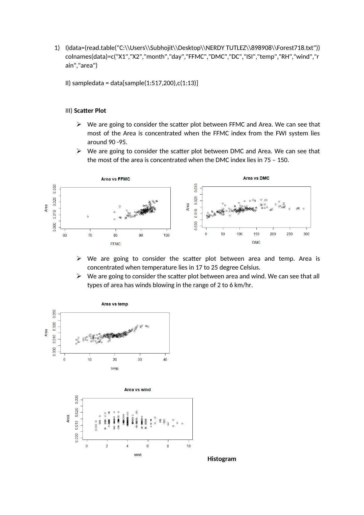
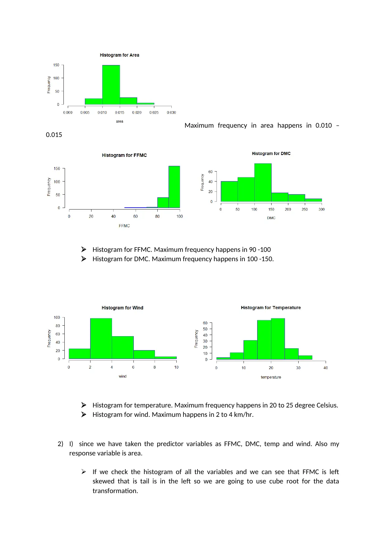
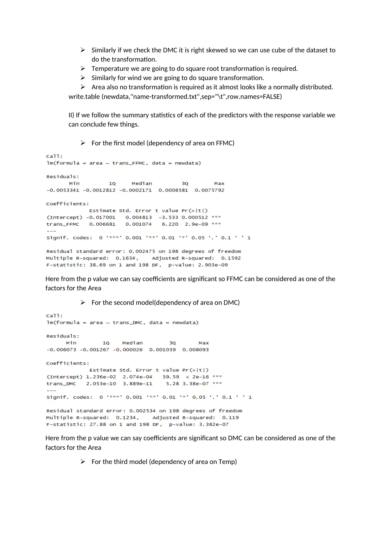
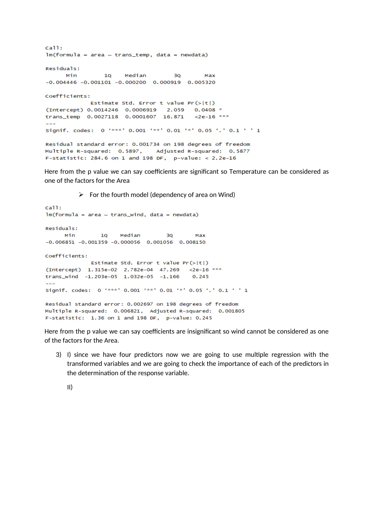
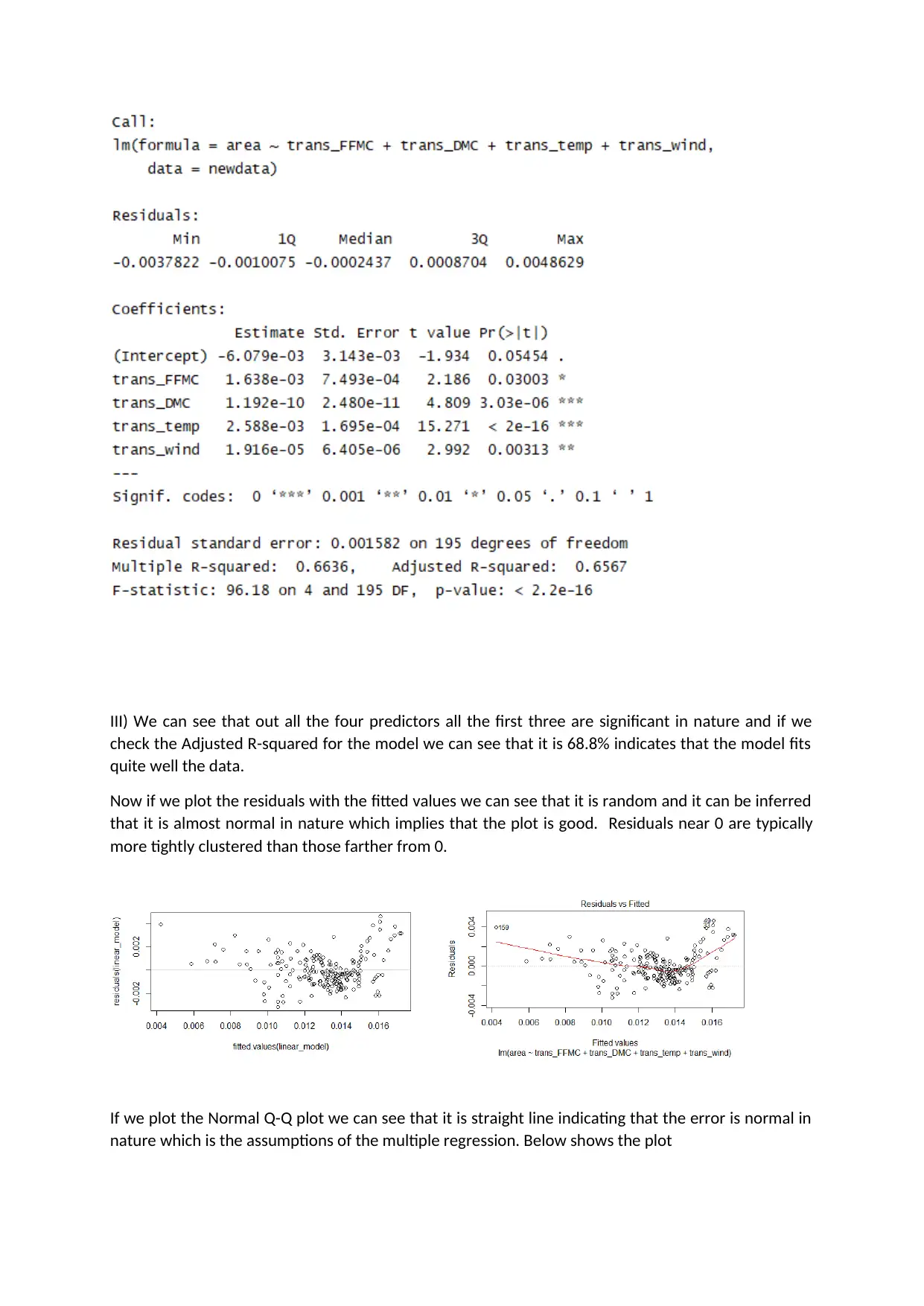
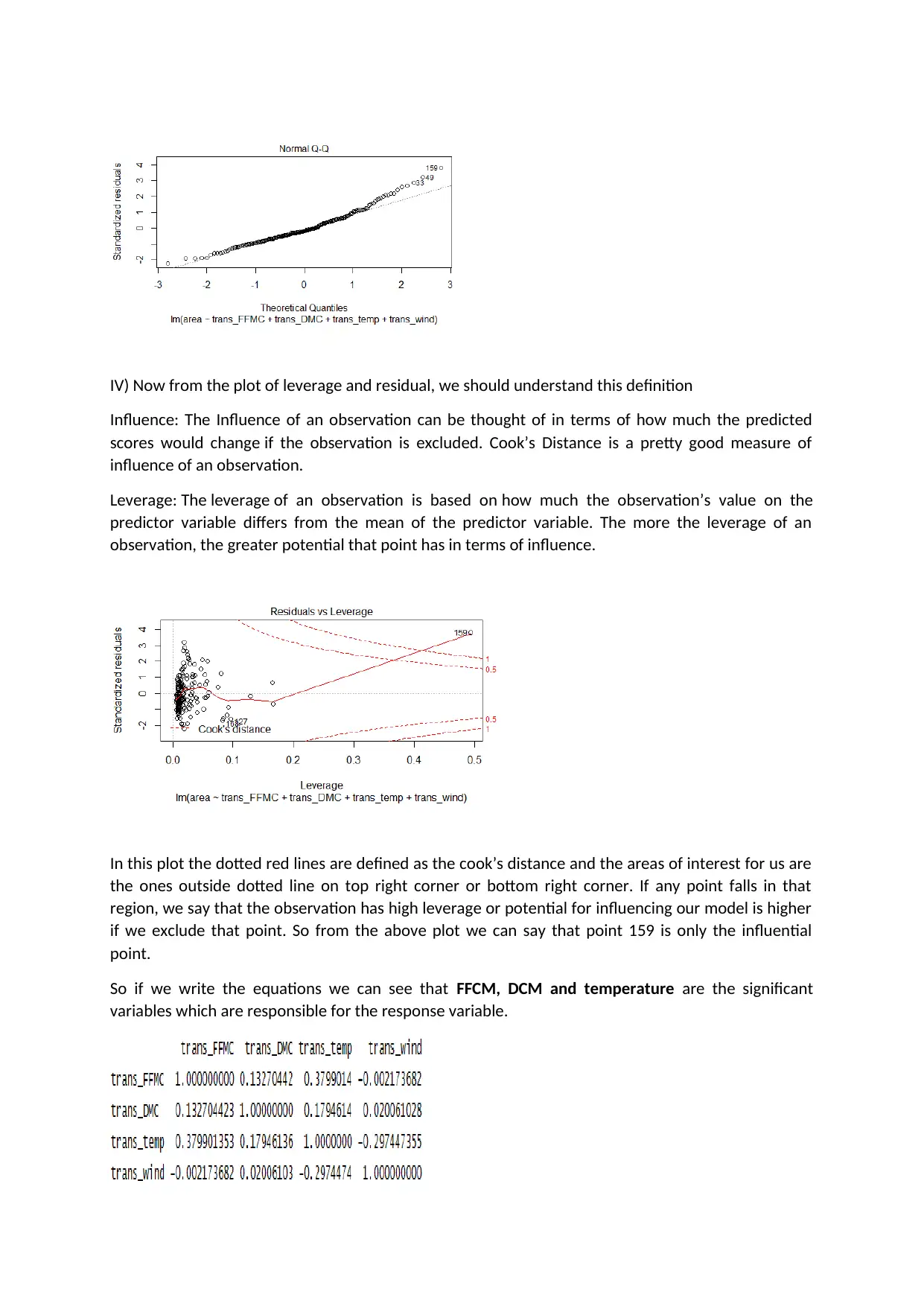
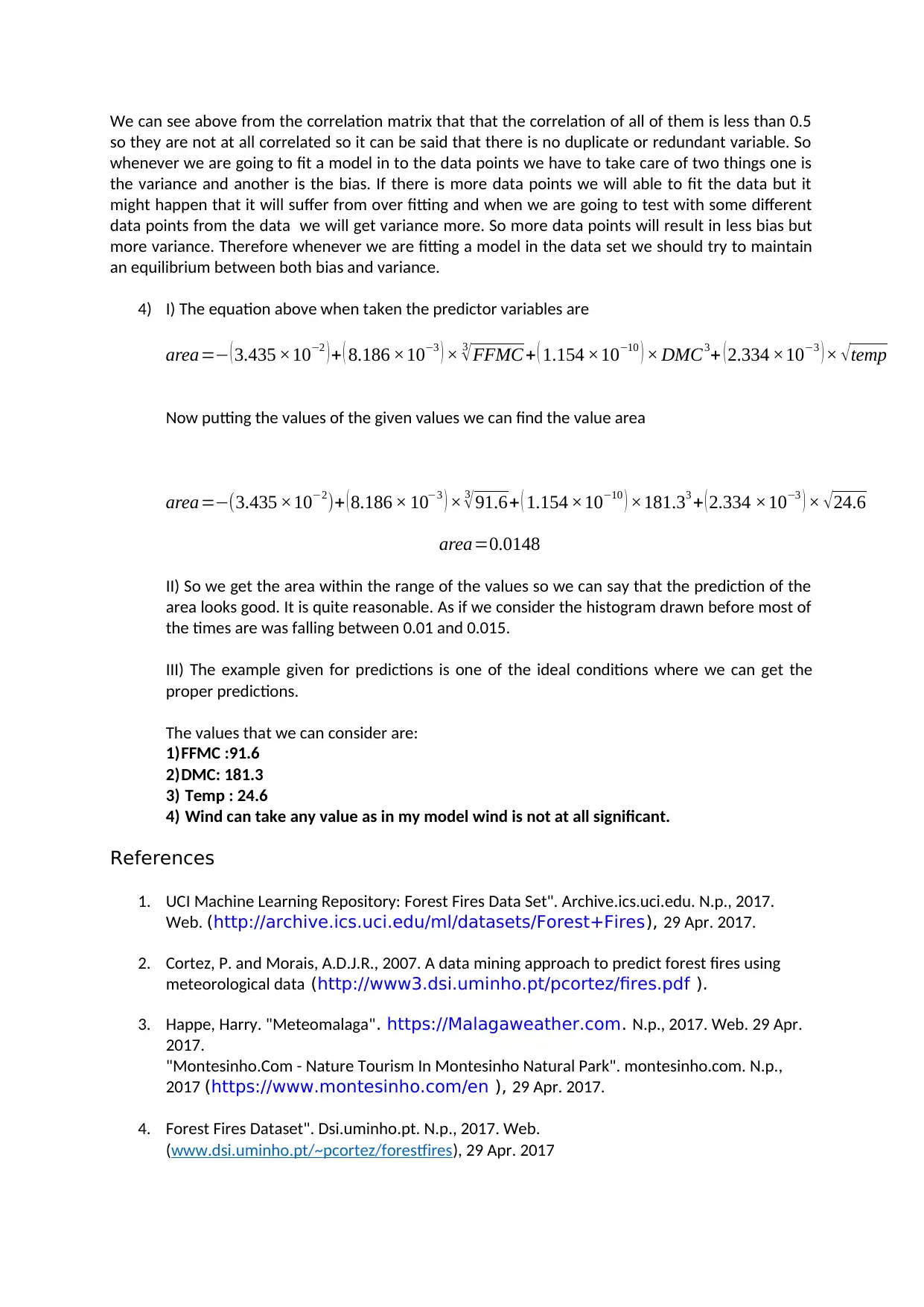
This project analyzes a forest fire dataset using R programming to predict the area burned by forest fires. The analysis includes data loading, cleaning, and exploratory data analysis (EDA) using scatter plots and histograms to understand the relationships between variables like FFMC, DMC, temperature, wind, and the area burned. Data transformation techniques, such as cube root, cube, and square root transformations, are applied to address skewness in the data. Multiple regression models are built to assess the significance of predictor variables in determining the area burned, with model diagnostics including residual plots and Q-Q plots to validate model assumptions. The project also discusses the concept of influence and leverage using Cook's Distance to identify influential data points. Finally, the project concludes with a prediction of the area burned based on given input values and provides references to the dataset and relevant publications.

1) I)data=(read.table("C:\\Users\\Subhojit\\Desktop\\NERDY TUTLEZ\\898908\\Forest718.txt"))
colnames(data)=c("X1","X2","month","day","FFMC","DMC","DC","ISI","temp","RH","wind","r
ain","area")
II) sampledata = data[sample(1:517,200),c(1:13)]
III) Scatter Plot
 We are going to consider the scatter plot between FFMC and Area. We can see that
most of the Area is concentrated when the FFMC index from the FWI system lies
around 90 -95.
 We are going to consider the scatter plot between DMC and Area. We can see that
the most of the area is concentrated when the DMC index lies in 75 – 150.
 We are going to consider the scatter plot between area and temp. Area is
concentrated when temperature lies in 17 to 25 degree Celsius.
 We are going to consider the scatter plot between area and wind. We can see that all
types of area has winds blowing in the range of 2 to 6 km/hr.
Histogram

Maximum frequency in area happens in 0.010 –
0.015
 Histogram for FFMC. Maximum frequency happens in 90 -100
 Histogram for DMC. Maximum frequency happens in 100 -150.
 Histogram for temperature. Maximum frequency happens in 20 to 25 degree Celsius.
 Histogram for wind. Maximum happens in 2 to 4 km/hr.
2) I) since we have taken the predictor variables as FFMC, DMC, temp and wind. Also my
response variable is area.
 If we check the histogram of all the variables and we can see that FFMC is left
skewed that is tail is in the left so we are going to use cube root for the data
transformation.

 Similarly if we check the DMC it is right skewed so we can use cube of the dataset to
do the transformation.
 Temperature we are going to do square root transformation is required.
 Similarly for wind we are going to do square transformation.
 Area also no transformation is required as it almost looks like a normally distributed.
write.table (newdata,"name-transformed.txt",sep="\t",row.names=FALSE)
II) If we follow the summary statistics of each of the predictors with the response variable we
can conclude few things.
 For the first model (dependency of area on FFMC)
Here from the p value we can say coefficients are significant so FFMC can be considered as one of the
factors for the Area
 For the second model(dependency of area on DMC)
Here from the p value we can say coefficients are significant so DMC can be considered as one of the
factors for the Area
 For the third model (dependency of area on Temp)

Here from the p value we can say coefficients are significant so Temperature can be considered as
one of the factors for the Area
 For the fourth model (dependency of area on Wind)
Here from the p value we can say coefficients are insignificant so wind cannot be considered as one
of the factors for the Area.
3) I) since we have four predictors now we are going to use multiple regression with the
transformed variables and we are going to check the importance of each of the predictors in
the determination of the response variable.
II)

III) We can see that out all the four predictors all the first three are significant in nature and if we
check the Adjusted R-squared for the model we can see that it is 68.8% indicates that the model fits
quite well the data.
Now if we plot the residuals with the fitted values we can see that it is random and it can be inferred
that it is almost normal in nature which implies that the plot is good. Residuals near 0 are typically
more tightly clustered than those farther from 0.
If we plot the Normal Q-Q plot we can see that it is straight line indicating that the error is normal in
nature which is the assumptions of the multiple regression. Below shows the plot

IV) Now from the plot of leverage and residual, we should understand this definition
Influence: The Influence of an observation can be thought of in terms of how much the predicted
scores would change if the observation is excluded. Cook’s Distance is a pretty good measure of
influence of an observation.
Leverage: The leverage of an observation is based on how much the observation’s value on the
predictor variable differs from the mean of the predictor variable. The more the leverage of an
observation, the greater potential that point has in terms of influence.
In this plot the dotted red lines are defined as the cook’s distance and the areas of interest for us are
the ones outside dotted line on top right corner or bottom right corner. If any point falls in that
region, we say that the observation has high leverage or potential for influencing our model is higher
if we exclude that point. So from the above plot we can say that point 159 is only the influential
point.
So if we write the equations we can see that FFCM, DCM and temperature are the significant
variables which are responsible for the response variable.

We can see above from the correlation matrix that that the correlation of all of them is less than 0.5
so they are not at all correlated so it can be said that there is no duplicate or redundant variable. So
whenever we are going to fit a model in to the data points we have to take care of two things one is
the variance and another is the bias. If there is more data points we will able to fit the data but it
might happen that it will suffer from over fitting and when we are going to test with some different
data points from the data we will get variance more. So more data points will result in less bias but
more variance. Therefore whenever we are fitting a model in the data set we should try to maintain
an equilibrium between both bias and variance.
4) I) The equation above when taken the predictor variables are
area=− ( 3.435 ×10−2 ) + ( 8.186 ×10−3 ) × 3
√FFMC + ( 1.154 ×10−10 ) × DMC3+ (2.334 ×10−3 ) × √temp
Now putting the values of the given values we can find the value area
area=−(3.435 ×10−2)+ ( 8.186 × 10−3 ) × 3
√91.6+ ( 1.154 ×10−10 ) ×181.33 + ( 2.334 ×10−3 ) × √24.6
area=0.0148
II) So we get the area within the range of the values so we can say that the prediction of the
area looks good. It is quite reasonable. As if we consider the histogram drawn before most of
the times are was falling between 0.01 and 0.015.
III) The example given for predictions is one of the ideal conditions where we can get the
proper predictions.
The values that we can consider are:
1)FFMC :91.6
2)DMC: 181.3
3) Temp : 24.6
4) Wind can take any value as in my model wind is not at all significant.
References
1. UCI Machine Learning Repository: Forest Fires Data Set". Archive.ics.uci.edu. N.p., 2017.
Web. (http://archive.ics.uci.edu/ml/datasets/Forest+Fires), 29 Apr. 2017.
2. Cortez, P. and Morais, A.D.J.R., 2007. A data mining approach to predict forest fires using
meteorological data (http://www3.dsi.uminho.pt/pcortez/fires.pdf ).
3. Happe, Harry. "Meteomalaga". https://Malagaweather.com. N.p., 2017. Web. 29 Apr.
2017.
"Montesinho.Com - Nature Tourism In Montesinho Natural Park". montesinho.com. N.p.,
2017 (https://www.montesinho.com/en ), 29 Apr. 2017.
4. Forest Fires Dataset". Dsi.uminho.pt. N.p., 2017. Web.
(www.dsi.uminho.pt/~pcortez/forestfires), 29 Apr. 2017