Understanding Security Market Line and Capital Market Line in Financial Management

This article explains the concepts of Security Market Line (SML) and Capital Market Line (CML) in Financial Management. It defines SML and CML, their equations, graphical representations, and limitations. It also highlights the differences between SML and CML, the importance of minimum variance portfolios, and the advantages of CAPM equation while calculating the rate of return. The article is relevant for students studying Financial Management in any college or university.

Running head: FINANCIAL MANAGEMENT
Financial Management
Name of the Student
Name of the University
Author note:

2FINANCIAL MANAGEMENT
Table of Contents
Introduction......................................................................................................................................3
Discussion........................................................................................................................................3
The SML:.....................................................................................................................................3
Definition:....................................................................................................................................3
Equation:......................................................................................................................................4
Graphical representation:.............................................................................................................4
Limitation....................................................................................................................................5
The CML:....................................................................................................................................5
Definition:....................................................................................................................................6
Equation:......................................................................................................................................6
Graphical representation:.............................................................................................................7
Limitation....................................................................................................................................8
The Fundamental difference between SML and CML................................................................9
The importance of minimum variance portfolios........................................................................9
The Advantages of CAPM equation whike calculating the rate of return.................................10
Conclusion.....................................................................................................................................11
References......................................................................................................................................12

3FINANCIAL MANAGEMENT
Introduction
A capital asset refers to the properties that are associated with the business of any kind.
The CAPM or the capital asset pricing model is the model that helps in the process of elaboration
of the link between the anticipated return of the asset and the systematic risk that is used widely
in the context of the stocks. In case of securities that are risk bearing, the CAPM is widely used.
This also helps in the generation of return that are expected for the assets and evaluating the cost
of capital.
In this context, the security market line refers to the line that is drawn that helps in
serving graphically representing the model of capital asset pricing. The SML also known as the
characteristics line which is visual capital pricing model that represents both risks and the return.
On the other hand, the CML stands for capital market line refers to the model that helps
in the pricing of asset CAPM mechanism. It represents the trade-off between return for portfolios
that are efficient and the various risks that are associated (Bodnar, Mazur and Okhrin 2017). It
can be said to be a theoretical concept which elaborates the various portfolios that efficiently
collaborate the rate of return that are free from risk as well as the risky assets market portfolio.
Discussion
The SML:
Definition:
The SML or the security market line refers to the optical depiction of the model of
capital asset pricing or CAPM. It represents the link between the return from security that is
expected and the associated risk. The measurement of risk is done by the beta coefficient (Chow,

4FINANCIAL MANAGEMENT
Kose and Li 2016). It can also be said in this context that, the representation of the SML shows
the anticipated return for any beta that is given or highlights the associated risk with any
expected return that is given.
Equation:
As highlighted in the above definition the SML is on the basis of the CAPM model that is
shown below:
E(Ri) = RF + βi × (E(RM) - RF)
Where, E(Ri) is an expected return of a security, RF is a risk-free rate, βi is a security’s
beta coefficient, and E(RM) is an expected market return.
Graphical representation:
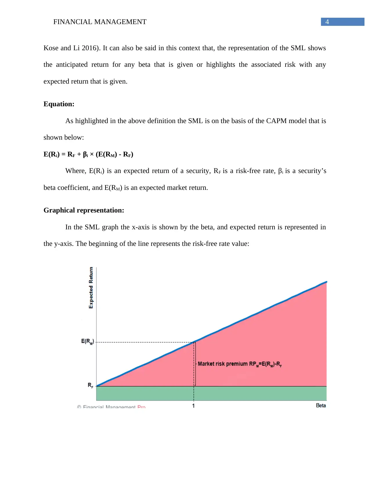
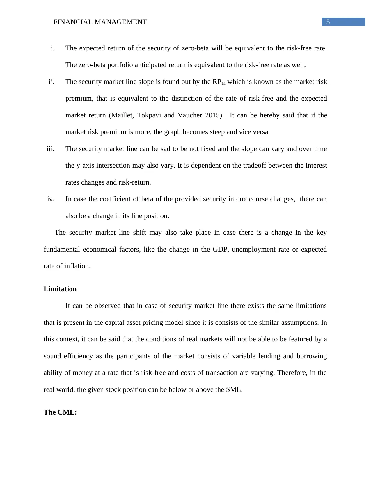
In the SML graph the x-axis is shown by the beta, and expected return is represented in
the y-axis. The beginning of the line represents the risk-free rate value:

5FINANCIAL MANAGEMENT
i. The expected return of the security of zero-beta will be equivalent to the risk-free rate.
The zero-beta portfolio anticipated return is equivalent to the risk-free rate as well.
ii. The security market line slope is found out by the RPM which is known as the market risk
premium, that is equivalent to the distinction of the rate of risk-free and the expected
market return (Maillet, Tokpavi and Vaucher 2015) . It can be hereby said that if the
market risk premium is more, the graph becomes steep and vice versa.
iii. The security market line can be sad to be not fixed and the slope can vary and over time
the y-axis intersection may also vary. It is dependent on the tradeoff between the interest
rates changes and risk-return.
iv. In case the coefficient of beta of the provided security in due course changes, there can
also be a change in its line position.
The security market line shift may also take place in case there is a change in the key
fundamental economical factors, like the change in the GDP, unemployment rate or expected
rate of inflation.
Limitation
It can be observed that in case of security market line there exists the same limitations
that is present in the capital asset pricing model since it is consists of the similar assumptions. In
this context, it can be said that the conditions of real markets will not be able to be featured by a
sound efficiency as the participants of the market consists of variable lending and borrowing
ability of money at a rate that is risk-free and costs of transaction are varying. Therefore, in the
real world, the given stock position can be below or above the SML.
The CML:

6FINANCIAL MANAGEMENT
Definition:
The CML or the Capital market line refers to the graph that shows the anticipated
portfolio return that consists of all the proportions that are possible between a risk-free asset and
market portfolio. In case the market portfolio is totally changed and carries the systematic risk
only, along with expecting a profit is equivalent to the anticipated return of the market. In
simpler terms, the calculation of the expected return of a specific portfolio (E(RC)) can be
evaluated as shown in te following equation:
E(Rc) = y × E(RM) + (1 – y) × RF
Here, the y market portfolio is a proportion, E(RM) stands for the expected market return
portfolio, the (1-y) refers to the risk-free asset proportion, and rate that is risk-free stands for RF.
The non leveraged portfolios return can be equal to or less than the market return in case the
market portfolio proportion of the is 100% or 1. However, the leveraged return portfolio can
considerably exceed the market return.
Equation:
As highlighted in the above definition the capital market line is on the basis of the CAPM
model that is shown below:
E(Rc) = RF + SDc
E(RM) - RF
SDM
Here, SDC stands for portfolio of standard deviation of C return; SDM refers to the a market
return standard deviation.
The CML slope is the reward to variability ratio (RVR).
RVR =
E(RM) - RF
SDM

7FINANCIAL MANAGEMENT
Graphical representation:
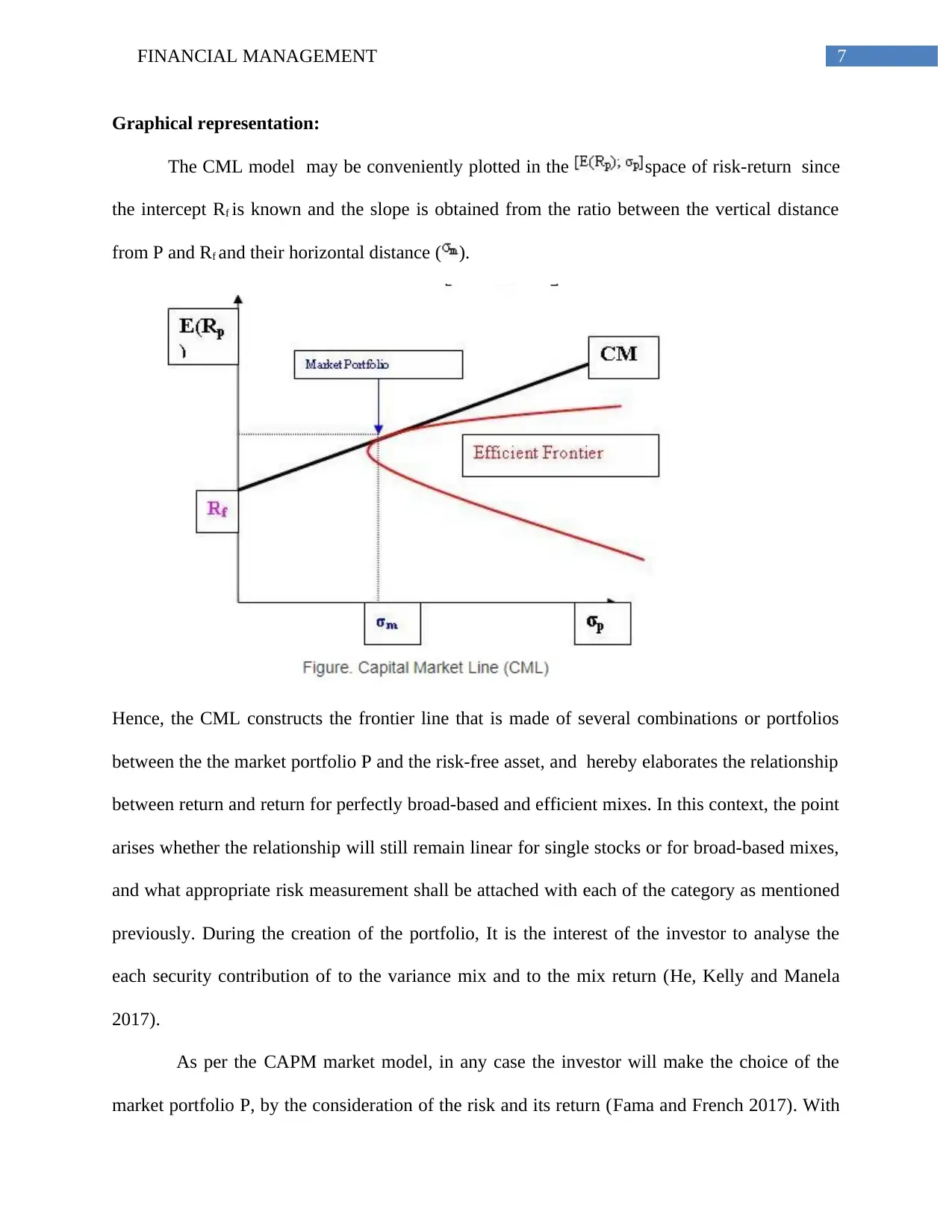
The CML model may be conveniently plotted in the space of risk-return since
the intercept Rf is known and the slope is obtained from the ratio between the vertical distance
from P and Rf and their horizontal distance ( ).
Hence, the CML constructs the frontier line that is made of several combinations or portfolios
between the the market portfolio P and the risk-free asset, and hereby elaborates the relationship
between return and return for perfectly broad-based and efficient mixes. In this context, the point
arises whether the relationship will still remain linear for single stocks or for broad-based mixes,
and what appropriate risk measurement shall be attached with each of the category as mentioned
previously. During the creation of the portfolio, It is the interest of the investor to analyse the
each security contribution of to the variance mix and to the mix return (He, Kelly and Manela
2017).
As per the CAPM market model, in any case the investor will make the choice of the
market portfolio P, by the consideration of the risk and its return (Fama and French 2017). With

8FINANCIAL MANAGEMENT
respect to the return, it is easy to observe the input that is given proportionally to E(Rm) by the
single asset regarding the own E(Ri).By ignoring the analytic derivation the quilibrium point can
be observed from the diagram given above that the contribution of asset should be compensated
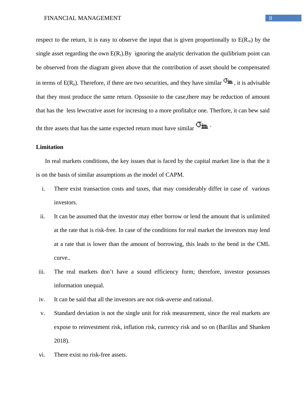
in terms of E(Rp). Therefore, if there are two securities, and they have similar , it is advisable
that they must produce the same return. Opssosite to the case,there may be reduction of amount
that has the less lewcrative asset for incresing to a more profitab;e one. Therfore, it can bew said
tht thre assets that has the same expected return must have similar `
Limitation
In real markets conditions, the key issues that is faced by the capital market line is that the it
is on the basis of similar assumptions as the model of CAPM.
i. There exist transaction costs and taxes, that may considerably differ in case of various
investors.
ii. It can be assumed that the investor may ether borrow or lend the amount that is unlimited
at the rate that is risk-free. In case of the conditions for real market the investors may lend
at a rate that is lower than the amount of borrowing, this leads to the bend in the CML
curve..
iii. The real markets don’t have a sound efficiency form; therefore, investor possesses
information unequal.
iv. It can be said that all the investors are not risk-averse and rational.
v. Standard deviation is not the single unit for risk measurement, since the real markets are
expose to reinvestment risk, inflation risk, currency risk and so on (Barillas and Shanken
2018).
vi. There exist no risk-free assets.

9FINANCIAL MANAGEMENT
Therefore, in real market condition the CML looks like a area that is fuzzy rather than a line that
is precise.
The Fundamental difference between SML and CML
Differences between CML and SML
Following represents the fundamental differences between SML and CML:
1. The Capital market line is the line that represents the return rate, it depends on rates of return
that are risk-free and risk level for a particular portfolio. The SML, that is known as the
Characteristic Line, refers to the graphical representation of the risk of the market and at a given
time risk(Bao, Diks and Li 2018).
2., In case of SML the risk factors are determined by the Beta coefficient and in case of CML
the standard deviation measures the risk.
3. The Security Market Line graphs define both non-efficient and efficient portfolios. However
in case of the CML the graphs define efficient portfolios
4. Hence it can be concluded that the CML is more superior at the time of measurement the
factors of risk.
The importance of minimum variance portfolios
The portfolio for minimum variance is the securities portfolio that minimizes the risk of
price for the overall portfolio. The volatility refers to the term that is more used commonly
instead of a variance in the community of investment; it is a statistical measure of a specific price
of the security movement that can be ups or downs.
The investment volatility can also be said to be interchangeable in meaning with its risk
of market. Hence, the more the investment volatility the up and down in price has wider swings

10FINANCIAL MANAGEMENT
that results in higher risk in market. Therefore, in case an investor opts for risk minimization,
they need to reduce the upasa and down in the market simultaneously.
The benefit of the minimum variance is that, there is a determination of the lower bond of the
efficient frontier. When there exists portfolios on the investment opportunity set to the right and
below the minimum variance portfolio, they are not efficient. That is, there is a portfolio with
the same level of a higher return and risk. None of the investor who is rational would ever make
an investment in a portfolio below the minimum variance portfolio.
The Advantages of CAPM equation while calculating the rate of return
The capital asset pricing model or the CAPM is the model that helps in the process of
elaboration of the relationship between the expected return of the asset and the systematic risk
that is used widely in the context of the stocks. In case of securities that are risk bearing, the
CAPM is widely used (Goh, Li, Ng and Yong 2015). This also helps in the generation of return
that are expected for the assets and evaluating the cost of capital. On the other hand the rate of
return refers to the loss or gain of investment over a time period that is specified, and is
expressed in terms of cost of investment percentage. The Investments gains are the income that is
received added with the capital gains that is realized on the sale of investment.
There are several advantages of the capital asset pricing model over other processes of evaluating
the needed return that explains the reason for it being popular for 40 years or more:
 The CML only considers the systematic risk that reflects a reality where most of the
investors have portfolios that have been diversified from which unsystematic risk has
been eliminated essentially.
 It refers to a relationship that is derived theoretically between the needed systematic risk
and return that is subject to frequent empirical testing and research.

11FINANCIAL MANAGEMENT
 It is seen generally as a a method that more efficient in calculating the cost of equity than
the growth model of dividend (DGM) in that it considers explicitly the level of the
company of systematic risk that is relative to the stock market on the whole (Barberis,
Greenwood, Jin and Shleifer 2015).
 It can be identified that the CML is clearly superior to the WACC in giving rates of
discount that can be used for appraisal of investment.
However, the CAPM suffers from various limitations and disadvantages that can be noted in a
balanced discussion of this vital theoretical model. In addition to this values need to be assigned
to the risk-free rate of return for using the model of CAPM that includes the the equity beta,
market return and the equity risk premium.
Conclusion
As per various researches it can be seen that the CAPM stands up fine to the various
criticism, even though the criticism against are increasing in present times. However, the model
of CAPM still remains a quite helpful item in the toolkit of financial management. In case of
securities that are risk bearing, the CAPM is widely used. This also helps in the generation of
return that are expected for the assets and evaluating the cost of capital. Hence from the above
discussion, it can be concluded that the CML is more superior at the time of measurement the
factors of risk.

12FINANCIAL MANAGEMENT
References
Bao, T., Diks, C. and Li, H., 2018. A generalized CAPM model with asymmetric power
distributed errors with an application to portfolio construction. Economic Modelling, 68, pp.611-
621.
Barberis, N., Greenwood, R., Jin, L. and Shleifer, A., 2015. X-CAPM: An extrapolative capital
asset pricing model. Journal of financial economics, 115(1), pp.1-24.
Barillas, F. and Shanken, J., 2018. Comparing asset pricing models. The Journal of
Finance, 73(2), pp.715-754.
Bodnar, T., Mazur, S. and Okhrin, Y., 2017. Bayesian estimation of the global minimum
variance portfolio. European Journal of Operational Research, 256(1), pp.292-307.
Chow, T.M., Kose, E. and Li, F., 2016. The impact of constraints on minimum-variance
portfolios. Financial Analysts Journal, 72(2), pp.52-70.
Fama, E.F. and French, K.R., 2017. International tests of a five-factor asset pricing
model. Journal of financial Economics, 123(3), pp.441-463.
Goh, B.W., Li, D., Ng, J. and Yong, K.O., 2015. Market pricing of banks’ fair value assets
reported under SFAS 157 since the 2008 financial crisis. Journal of Accounting and Public
Policy, 34(2), pp.129-145.
He, Z., Kelly, B. and Manela, A., 2017. Intermediary asset pricing: New evidence from many
asset classes. Journal of Financial Economics, 126(1), pp.1-35.
Maillet, B., Tokpavi, S. and Vaucher, B., 2015. Global minimum variance portfolio optimisation
under some model risk: A robust regression-based approach. European Journal of Operational
Research, 244(1), pp.289-299.

13FINANCIAL MANAGEMENT
McDonald, J., Michelfelder, R.A. and Theodossiou, P., 2015. Robust regression estimation
methods and intercept bias: A capital asset pricing model application.
Nasiri, M., Alishah, A.Y., Sayyahmelli, S.A.S. and Karimi, A., 2017. Estimating Expected
Return based on Capital Asset Pricing Model compared with Stock Interest Rate at Tehran Stock
Exchange. HELIX, 7(2), pp.1406-1415.
Nghiem, L., 2015. Risk-return relationship: An empirical study of different statistical methods
for estimating the Capital Asset Pricing Models (CAPM) and the Fama-French model for large
cap stocks. arXiv preprint arXiv:1511.07101.
Sumalatha, V. and Santhi, R., 2017. Deployment of Classification Approach for Sensing Stress
of Juvenile Using CAPM Model.
Wang, T., 2017. Revealed Preferences of Mutual Fund Investors in Good and Bad Times.
Zabarankin, M., Pavlikov, K. and Uryasev, S., 2014. Capital asset pricing model (CAPM) with
drawdown measure. European Journal of Operational Research, 234(2), pp.508-517.
Zhou, T. and Liu, H., 2018. Empirical study on CAPM model of China stock market.