SG1022 Quantitative Methods: Probability, Regression and F-Test
VerifiedAdded on 2023/06/10
|14
|2898
|117
Homework Assignment
AI Summary
This assignment focuses on applying quantitative methods to analyze data and solve problems related to probability, regression, and financial calculations. It includes constructing joint probability tables to determine probabilities of events, performing regression analysis to develop equations for predicting GDP based on population and tax revenue, conducting F-tests and t-tests to assess the significance of regression models and individual variables, and calculating compounded interest annually and quarterly. The solutions demonstrate the application of statistical concepts and formulas to real-world scenarios, providing insights into data analysis and decision-making. Desklib offers this assignment as a valuable resource for students seeking to enhance their understanding of quantitative methods and improve their problem-solving skills.
SG1022 Quantitative
Methods
Methods
Paraphrase This Document
Need a fresh take? Get an instant paraphrase of this document with our AI Paraphraser
Contents
QUESTION 1..................................................................................................................................4
a) Develop a joint probability table for the data on occupation of workers................................4
b) Determine what is the probability of a female worker being a civil engineer........................4
c) Determine what is the probability of a male worker being a Chief Executive Officer...........4
d) Determine whether occupation is independent of gender and justify your answer with a
probability calculation. Please show your calculations...............................................................4
Question 2........................................................................................................................................5
a. Develop a joint probability table and show the marginal probabilities of men, women, part
time and full time. Comment on the results.................................................................................5
b) If a person is working in full time, what is the probability given that the selected person is a
male..............................................................................................................................................5
c) If a person works part time, what is the probability given that the selected person is a
female..........................................................................................................................................5
d) Let A denote the event that a person is a full time and let B be the event that the person is a
female. Determine whether A and B are independent events and justify the answer..................6
Question 3........................................................................................................................................6
Develop the regression equation that can be used to predict the GDP by Population and Tax
received........................................................................................................................................6
b) Provide an explanation for the regression coefficients b1 and b2 from the regression
equation........................................................................................................................................7
c) Use the estimated regression equation developed in part (a) to estimate the GDP if the
population is 67886011 and the tax received 249521.................................................................8
d) Explain whether the regression equation developed in part (a) provides a good fit for the
observed data by interpreting the coefficient of determination...................................................8
Question 4........................................................................................................................................9
a) Conduct an F-test to determine the overall significance of the regression model...................9
b) Use the t- test to determine the significance of each independent variable namely Population
and Tax Received. Explain the conclusion at the 0.05 level of significance...............................9
Question 5......................................................................................................................................10
a) Compounded annual and explain..........................................................................................10
b) Compounded quarterly and explain......................................................................................10
Question 6......................................................................................................................................11
Question 7......................................................................................................................................12
REFERENCES..............................................................................................................................13
⊘ This is a preview!⊘
Do you want full access?
Subscribe today to unlock all pages.

Trusted by 1+ million students worldwide
QUESTION 1
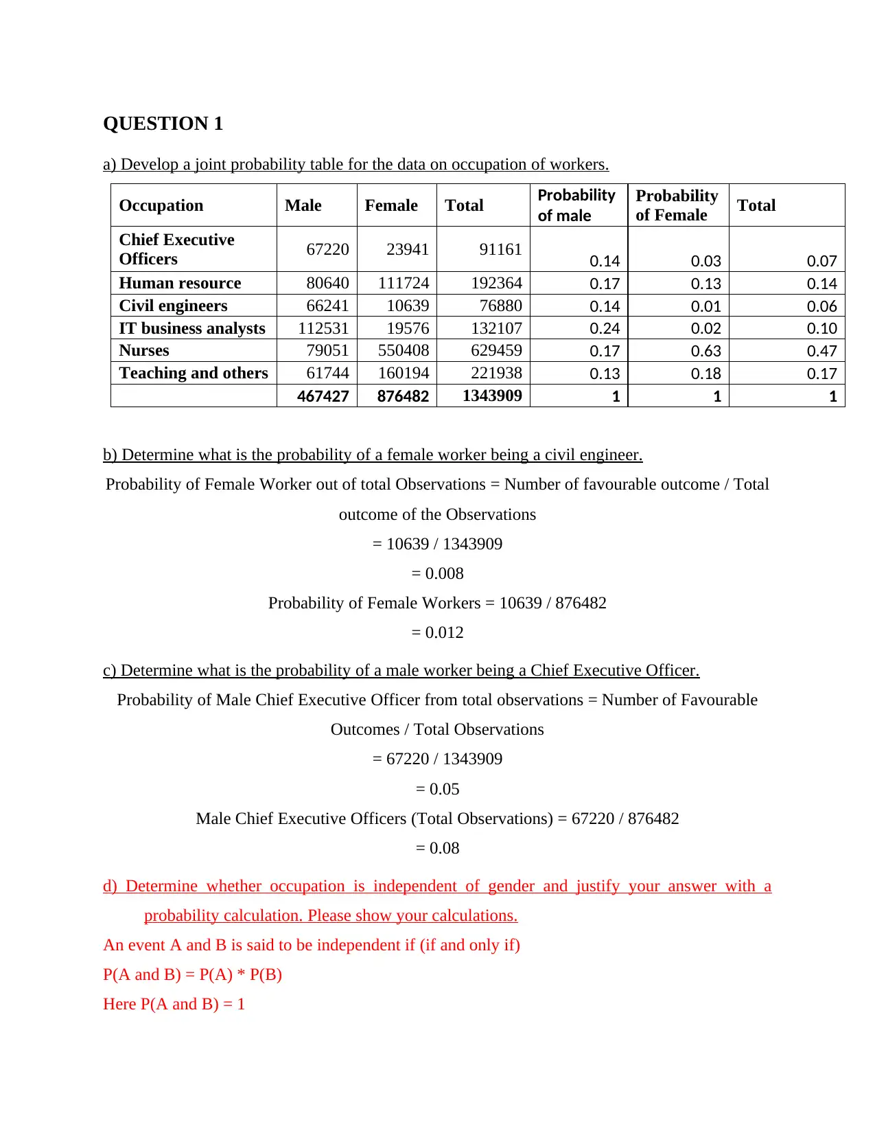
a) Develop a joint probability table for the data on occupation of workers.
Occupation Male Female Total Probability
of male
Probability
of Female Total
Chief Executive
Officers 67220 23941 91161 0.14 0.03 0.07
Human resource 80640 111724 192364 0.17 0.13 0.14
Civil engineers 66241 10639 76880 0.14 0.01 0.06
IT business analysts 112531 19576 132107 0.24 0.02 0.10
Nurses 79051 550408 629459 0.17 0.63 0.47
Teaching and others 61744 160194 221938 0.13 0.18 0.17
467427 876482 1343909 1 1 1
b) Determine what is the probability of a female worker being a civil engineer.
Probability of Female Worker out of total Observations = Number of favourable outcome / Total
outcome of the Observations
= 10639 / 1343909
= 0.008
Probability of Female Workers = 10639 / 876482
= 0.012
c) Determine what is the probability of a male worker being a Chief Executive Officer.
Probability of Male Chief Executive Officer from total observations = Number of Favourable
Outcomes / Total Observations
= 67220 / 1343909
= 0.05
Male Chief Executive Officers (Total Observations) = 67220 / 876482
= 0.08
d) Determine whether occupation is independent of gender and justify your answer with a
probability calculation. Please show your calculations.
An event A and B is said to be independent if (if and only if)
P(A and B) = P(A) * P(B)
Here P(A and B) = 1
Paraphrase This Document
Need a fresh take? Get an instant paraphrase of this document with our AI Paraphraser
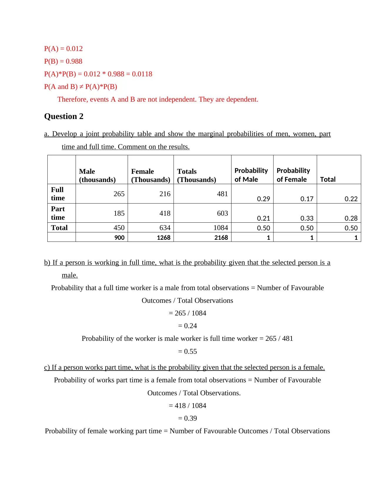
P(A) = 0.012
P(B) = 0.988
P(A)*P(B) = 0.012 * 0.988 = 0.0118
P(A and B) ≠ P(A)*P(B)
Therefore, events A and B are not independent. They are dependent.
Question 2
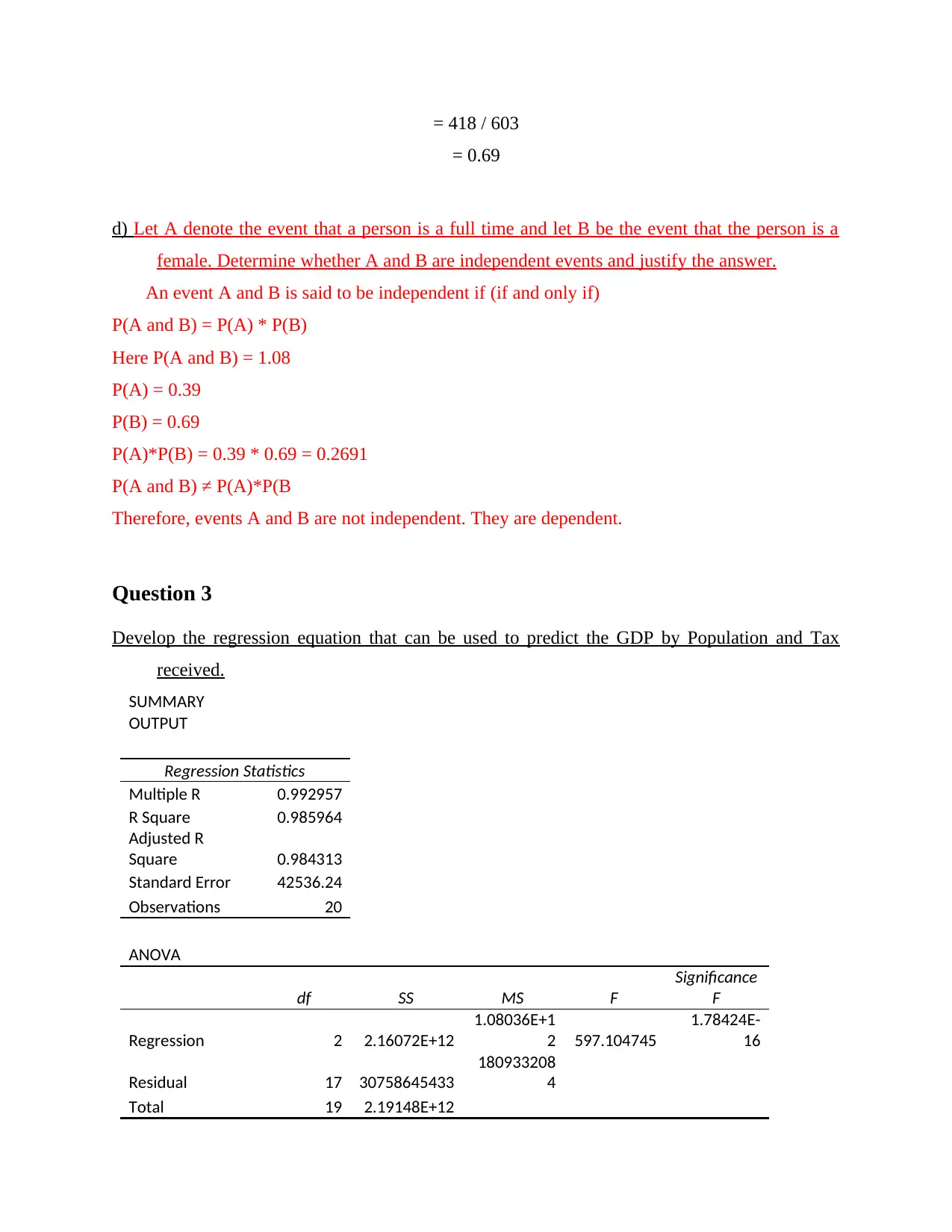
a. Develop a joint probability table and show the marginal probabilities of men, women, part
time and full time. Comment on the results.
Male
(thousands)
Female
(Thousands)
Totals
(Thousands)
Probability
of Male
Probability
of Female Total
Full
time 265 216 481 0.29 0.17 0.22
Part
time 185 418 603 0.21 0.33 0.28
Total 450 634 1084 0.50 0.50 0.50
900 1268 2168 1 1 1
b) If a person is working in full time, what is the probability given that the selected person is a
male.
Probability that a full time worker is a male from total observations = Number of Favourable
Outcomes / Total Observations
= 265 / 1084
= 0.24
Probability of the worker is male worker is full time worker = 265 / 481
= 0.55
c) If a person works part time, what is the probability given that the selected person is a female.
Probability of works part time is a female from total observations = Number of Favourable
Outcomes / Total Observations.
= 418 / 1084
= 0.39
Probability of female working part time = Number of Favourable Outcomes / Total Observations
= 418 / 603
= 0.69
d) Let A denote the event that a person is a full time and let B be the event that the person is a
female. Determine whether A and B are independent events and justify the answer.
An event A and B is said to be independent if (if and only if)
P(A and B) = P(A) * P(B)
Here P(A and B) = 1.08
P(A) = 0.39
P(B) = 0.69
P(A)*P(B) = 0.39 * 0.69 = 0.2691
P(A and B) ≠ P(A)*P(B
Therefore, events A and B are not independent. They are dependent.
Question 3
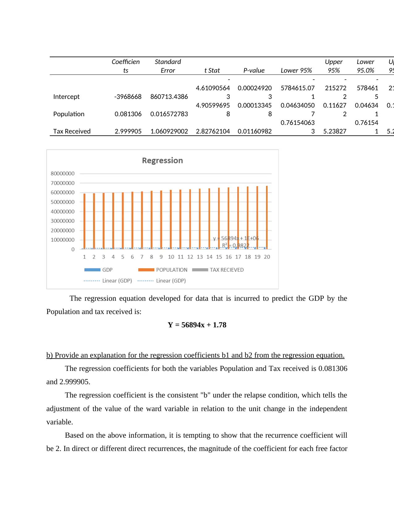
Develop the regression equation that can be used to predict the GDP by Population and Tax
received.
SUMMARY
OUTPUT
Regression Statistics
Multiple R 0.992957
R Square 0.985964
Adjusted R
Square 0.984313
Standard Error 42536.24
Observations 20
ANOVA
df SS MS F
Significance
F
Regression 2 2.16072E+12
1.08036E+1
2 597.104745
1.78424E-
16
Residual 17 30758645433
180933208
4
Total 19 2.19148E+12
⊘ This is a preview!⊘
Do you want full access?
Subscribe today to unlock all pages.

Trusted by 1+ million students worldwide
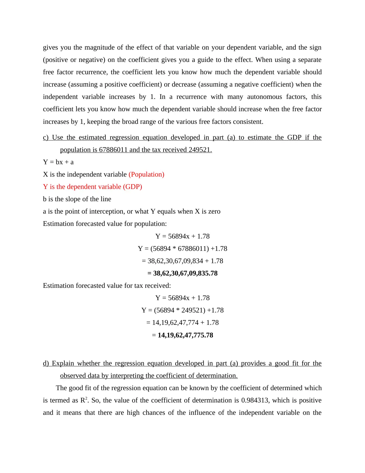
Coefficien
ts
Standard
Error t Stat P-value Lower 95%
Upper
95%
Lower
95.0%
Up
95
Intercept -3968668 860713.4386
-
4.61090564
3
0.00024920
3
-
5784615.07
1
-
215272
2
-
578461
5
21
Population 0.081306 0.016572783
4.90599695
8
0.00013345
8
0.04634050
7
0.11627
2
0.04634
1
0.1
Tax Received 2.999905 1.060929002 2.82762104 0.01160982
0.76154063
3 5.23827
0.76154
1 5.2
The regression equation developed for data that is incurred to predict the GDP by the
Population and tax received is:
Y = 56894x + 1.78
b) Provide an explanation for the regression coefficients b1 and b2 from the regression equation.
The regression coefficients for both the variables Population and Tax received is 0.081306
and 2.999905.
The regression coefficient is the consistent "b" under the relapse condition, which tells the
adjustment of the value of the ward variable in relation to the unit change in the independent
variable.
Based on the above information, it is tempting to show that the recurrence coefficient will
be 2. In direct or different direct recurrences, the magnitude of the coefficient for each free factor
Paraphrase This Document
Need a fresh take? Get an instant paraphrase of this document with our AI Paraphraser
gives you the magnitude of the effect of that variable on your dependent variable, and the sign
(positive or negative) on the coefficient gives you a guide to the effect. When using a separate
free factor recurrence, the coefficient lets you know how much the dependent variable should
increase (assuming a positive coefficient) or decrease (assuming a negative coefficient) when the
independent variable increases by 1. In a recurrence with many autonomous factors, this
coefficient lets you know how much the dependent variable should increase when the free factor
increases by 1, keeping the broad range of the various free factors consistent.
c) Use the estimated regression equation developed in part (a) to estimate the GDP if the
population is 67886011 and the tax received 249521.
Y = bx + a
X is the independent variable (Population)
Y is the dependent variable (GDP)
b is the slope of the line
a is the point of interception, or what Y equals when X is zero
Estimation forecasted value for population:
Y = 56894x + 1.78
Y = (56894 * 67886011) +1.78
= 38,62,30,67,09,834 + 1.78
= 38,62,30,67,09,835.78
Estimation forecasted value for tax received:
Y = 56894x + 1.78
Y = (56894 * 249521) +1.78
= 14,19,62,47,774 + 1.78
= 14,19,62,47,775.78
d) Explain whether the regression equation developed in part (a) provides a good fit for the
observed data by interpreting the coefficient of determination.
The good fit of the regression equation can be known by the coefficient of determined which
is termed as R2. So, the value of the coefficient of determination is 0.984313, which is positive
and it means that there are high chances of the influence of the independent variable on the
dependent variable. It means that 98.4313 % changes are there that GDP influences the variable
named Population and Tax received.
Question 4
a) Conduct an F-test to determine the overall significance of the regression model.
F-Test Two-Sample for Variances
Population
Tax
Received
Mean 63013670 178552.45
Variance
7.00435E+1
2
170917381
7
Observations 20 20
df 19 19
F
4098.09251
9
P(F<=f) one-tail 2.25966E-30
F Critical one-tail
2.16825160
1
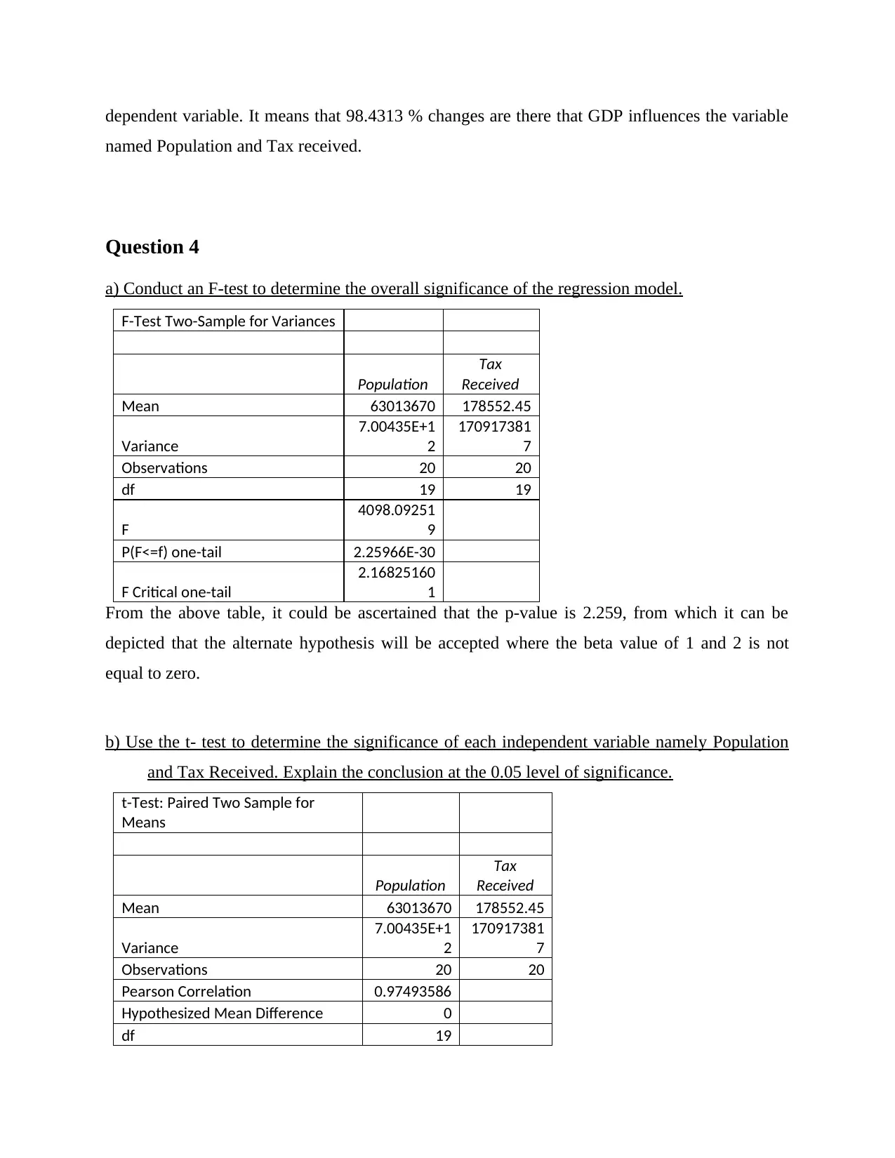
From the above table, it could be ascertained that the p-value is 2.259, from which it can be
depicted that the alternate hypothesis will be accepted where the beta value of 1 and 2 is not
equal to zero.
b) Use the t- test to determine the significance of each independent variable namely Population
and Tax Received. Explain the conclusion at the 0.05 level of significance.
t-Test: Paired Two Sample for
Means
Population
Tax
Received
Mean 63013670 178552.45
Variance
7.00435E+1
2
170917381
7
Observations 20 20
Pearson Correlation 0.97493586
Hypothesized Mean Difference 0
df 19
⊘ This is a preview!⊘
Do you want full access?
Subscribe today to unlock all pages.

Trusted by 1+ million students worldwide
t Stat
107.819097
5
P(T<=t) one-tail
2.99465E-
28
t Critical one-tail
1.72913281
2
P(T<=t) two-tail
5.98929E-
28
t Critical two-tail
2.09302405
4
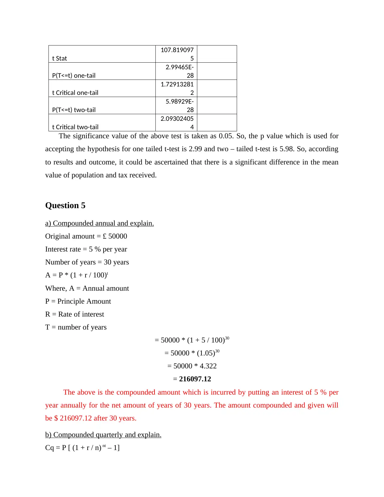
The significance value of the above test is taken as 0.05. So, the p value which is used for
accepting the hypothesis for one tailed t-test is 2.99 and two – tailed t-test is 5.98. So, according
to results and outcome, it could be ascertained that there is a significant difference in the mean
value of population and tax received.
Question 5
a) Compounded annual and explain.
Original amount = £ 50000
Interest rate = 5 % per year
Number of years = 30 years
A = P * (1 + r / 100)t
Where, A = Annual amount
P = Principle Amount
R = Rate of interest
T = number of years
= 50000 * (1 + 5 / 100)30
= 50000 * (1.05)30
= 50000 * 4.322
= 216097.12
The above is the compounded amount which is incurred by putting an interest of 5 % per
year annually for the net amount of years of 30 years. The amount compounded and given will
be $ 216097.12 after 30 years.
b) Compounded quarterly and explain.
Cq = P [ (1 + r / n) nt – 1]
Paraphrase This Document
Need a fresh take? Get an instant paraphrase of this document with our AI Paraphraser
Where, P = Principle Amount
R = rate of interest
T = number of years
N = Number of quarters
Cq = Compounded Quarterly
= 50000 * [(1 + 0.05 / 4)4 * 30]
= 50000 * [(1 + 0.0125)120]
= 50000 * [1.0125]120
= 50000 * 6.523
= 222010.66
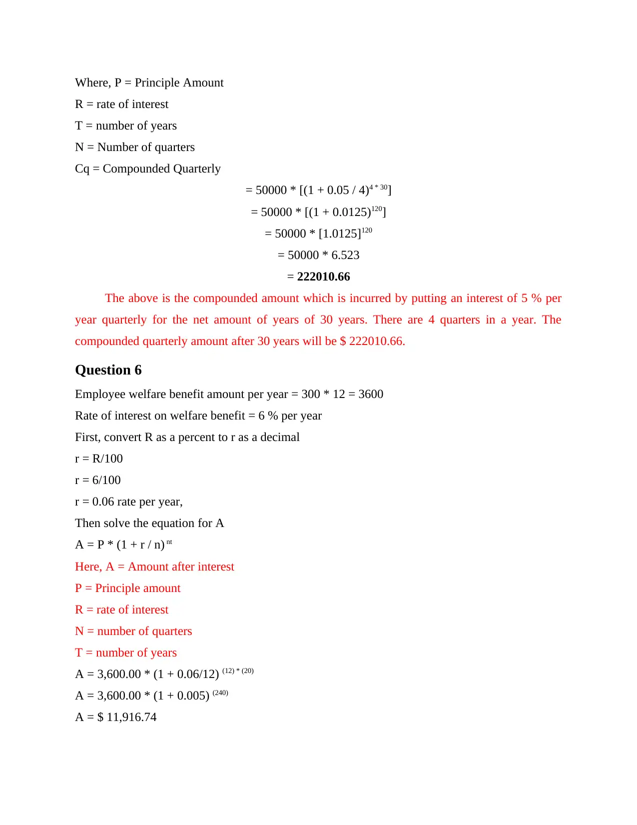
The above is the compounded amount which is incurred by putting an interest of 5 % per
year quarterly for the net amount of years of 30 years. There are 4 quarters in a year. The
compounded quarterly amount after 30 years will be $ 222010.66.
Question 6
Employee welfare benefit amount per year = 300 * 12 = 3600
Rate of interest on welfare benefit = 6 % per year
First, convert R as a percent to r as a decimal
r = R/100
r = 6/100
r = 0.06 rate per year,
Then solve the equation for A
A = P * (1 + r / n) nt
Here, A = Amount after interest
P = Principle amount
R = rate of interest
N = number of quarters
T = number of years
A = 3,600.00 * (1 + 0.06/12) (12) * (20)
A = 3,600.00 * (1 + 0.005) (240)
A = $ 11,916.74
R = rate of interest
T = number of years
N = Number of quarters
Cq = Compounded Quarterly
= 50000 * [(1 + 0.05 / 4)4 * 30]
= 50000 * [(1 + 0.0125)120]
= 50000 * [1.0125]120
= 50000 * 6.523
= 222010.66
The above is the compounded amount which is incurred by putting an interest of 5 % per
year quarterly for the net amount of years of 30 years. There are 4 quarters in a year. The
compounded quarterly amount after 30 years will be $ 222010.66.
Question 6
Employee welfare benefit amount per year = 300 * 12 = 3600
Rate of interest on welfare benefit = 6 % per year
First, convert R as a percent to r as a decimal
r = R/100
r = 6/100
r = 0.06 rate per year,
Then solve the equation for A
A = P * (1 + r / n) nt
Here, A = Amount after interest
P = Principle amount
R = rate of interest
N = number of quarters
T = number of years
A = 3,600.00 * (1 + 0.06/12) (12) * (20)
A = 3,600.00 * (1 + 0.005) (240)
A = $ 11,916.74
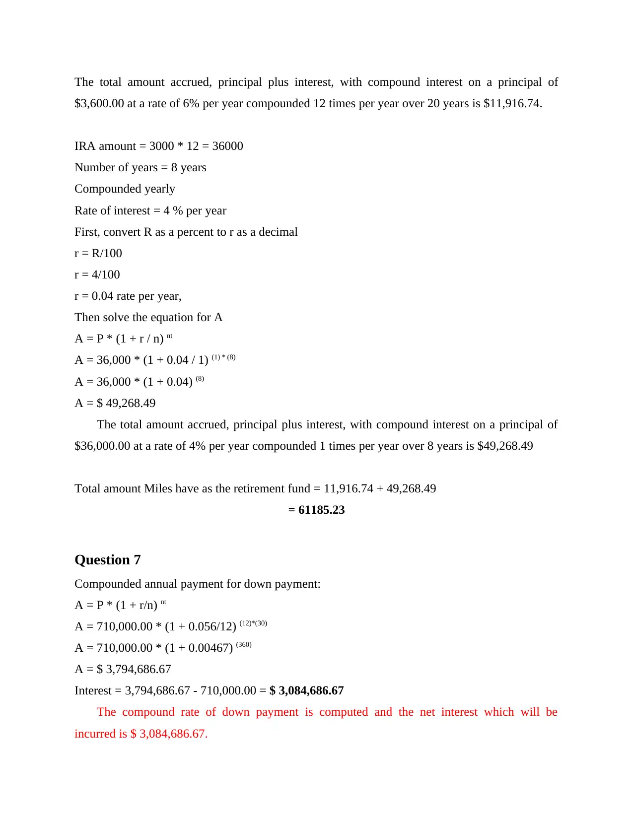
The total amount accrued, principal plus interest, with compound interest on a principal of
$3,600.00 at a rate of 6% per year compounded 12 times per year over 20 years is $11,916.74.
IRA amount = 3000 * 12 = 36000
Number of years = 8 years
Compounded yearly
Rate of interest = 4 % per year
First, convert R as a percent to r as a decimal
r = R/100
r = 4/100
r = 0.04 rate per year,
Then solve the equation for A
A = P * (1 + r / n) nt
A = 36,000 * (1 + 0.04 / 1) (1) * (8)
A = 36,000 * (1 + 0.04) (8)
A = $ 49,268.49
The total amount accrued, principal plus interest, with compound interest on a principal of
$36,000.00 at a rate of 4% per year compounded 1 times per year over 8 years is $49,268.49
Total amount Miles have as the retirement fund = 11,916.74 + 49,268.49
= 61185.23
Question 7
Compounded annual payment for down payment:
A = P * (1 + r/n) nt
A = 710,000.00 * (1 + 0.056/12) (12)*(30)
A = 710,000.00 * (1 + 0.00467) (360)
A = $ 3,794,686.67
Interest = 3,794,686.67 - 710,000.00 = $ 3,084,686.67
The compound rate of down payment is computed and the net interest which will be
incurred is $ 3,084,686.67.
⊘ This is a preview!⊘
Do you want full access?
Subscribe today to unlock all pages.

Trusted by 1+ million students worldwide
1 out of 14
Your All-in-One AI-Powered Toolkit for Academic Success.
+13062052269
info@desklib.com
Available 24*7 on WhatsApp / Email
![[object Object]](/_next/static/media/star-bottom.7253800d.svg)
Unlock your academic potential
Copyright © 2020–2025 A2Z Services. All Rights Reserved. Developed and managed by ZUCOL.

