Linear Regression Analysis of Sales and Consumption Survey Data

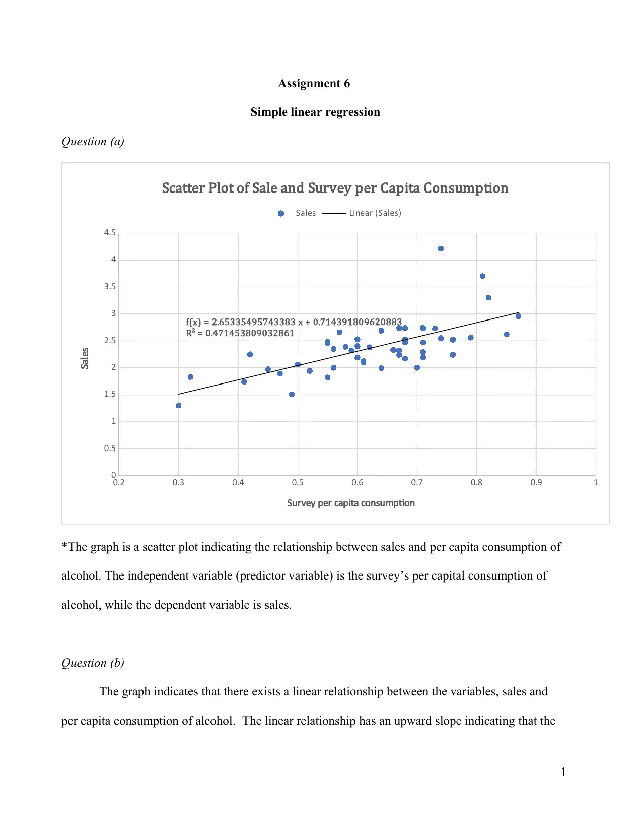
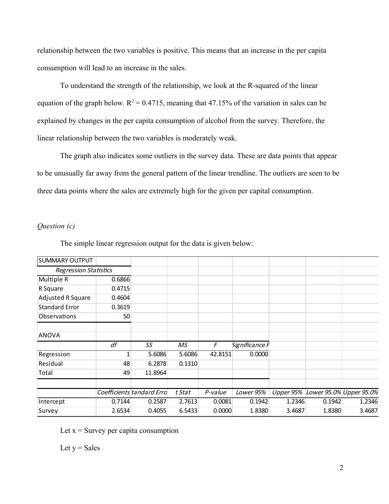
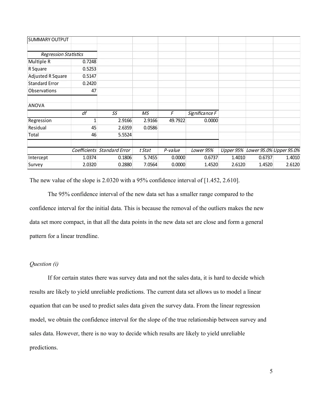
This assignment solution presents a detailed analysis of sales data using simple linear regression. It begins with a scatter plot illustrating the relationship between sales and per capita consumption of alcohol, identifying the independent and dependent variables. The solution then discusses the linear relationship, R-squared value, and the presence of outliers. It includes the simple linear regression output, the line of best fit, and interpretations of the slope and intercept. The analysis covers the coefficient of determination, hypothesis testing to determine the significance of the linear relationship, and the calculation of a 95% confidence interval for the slope. Finally, the assignment addresses the impact of removing outliers on the regression results and the reliability of predictions when sales data is missing, providing a comprehensive statistical analysis of the provided data.

Assignment 6
Simple linear regression
Question (a)
0.2 0.3 0.4 0.5 0.6 0.7 0.8 0.9 1
0
0.5
1
1.5
2
2.5
3
3.5
4
4.5
f(x) = 2.65335495743383 x + 0.714391809620883
R² = 0.471453809032861
Scatter Plot of Sale and Survey per Capita Consumption
Sales Linear (Sales)
Survey per capita consumption
Sales
*The graph is a scatter plot indicating the relationship between sales and per capita consumption of
alcohol. The independent variable (predictor variable) is the survey’s per capital consumption of
alcohol, while the dependent variable is sales.
Question (b)
The graph indicates that there exists a linear relationship between the variables, sales and
per capita consumption of alcohol. The linear relationship has an upward slope indicating that the
1

relationship between the two variables is positive. This means that an increase in the per capita
consumption will lead to an increase in the sales.
To understand the strength of the relationship, we look at the R-squared of the linear
equation of the graph below. R2 = 0.4715, meaning that 47.15% of the variation in sales can be
explained by changes in the per capita consumption of alcohol from the survey. Therefore, the
linear relationship between the two variables is moderately weak.
The graph also indicates some outliers in the survey data. These are data points that appear
to be unusually far away from the general pattern of the linear trendline. The outliers are seen to be
three data points where the sales are extremely high for the given per capital consumption.
Question (c)
The simple linear regression output for the data is given below:
SUMMARY OUTPUT
Regression Statistics
Multiple R 0.6866
R Square 0.4715
Adjusted R Square 0.4604
Standard Error 0.3619
Observations 50
ANOVA
df
SS MS F Significance F
Regression 1 5.6086 5.6086 42.8151 0.0000
Residual 48 6.2878 0.1310
Total 49 11.8964
CoefficientsStandard Error t Stat P-value Lower 95% Upper 95% Lower 95.0% Upper 95.0%
Intercept 0.7144 0.2587 2.7613 0.0081 0.1942 1.2346 0.1942 1.2346
Survey 2.6534 0.4055 6.5433 0.0000 1.8380 3.4687 1.8380 3.4687
Line of best fit:
Let x = Survey per capita consumption
Let y = Sales
2

^y will denote the expected sales when the per capita consumption is x.
 Line of best fit: ^y=0.7144+2.6534
Question (d)
The value of the slope for the line of best fit is 2.6534; This means if the per capita
consumption increases by 1, then the model predicts that the sales will increase by 2.6534. The
value of the intercept for the line of best fit is 0.7144; This means if the per capita consumption is 0,
then the model predicts the sales will be 0.7144.
The intercept does not have a reliable interpretation because it is unrealistic to have any
sales recorded if there is no consumption of alcohol across the states.
Question (e)
The coefficient of determination, R2 is used to assess the ability of the model to predict an
outcome. In this case, the value of the coefficient of determination of the simple linear regression
model was found to be, R2 = 0.4715. Hence, 47.15% of the variations in Sales (the dependent
variable) can be predicted by a simple linear regression and per capita consumption (independent
variable).
Question (f)
The test whether there is a significant linear relationship between the survey data and the
Sales data, at 5% level of significance, we first formulate the hypothesis as:
H0: 1 = 0
H1: 1 ≠ 0
3

The decision rule is to reject the null hypothesis, if p-value is less than the significance
level.
The p-value = 0.0000
Level of significance = 0.05
 0.00 < 0.05, Reject null hypothesis. Hence, there is sufficient evidence to conclude that
there is a significant linear relationship between the survey data and the sales data, at 95%
confidence level.
Question (g)
The 95% confidence interval for the slope of the true relationship between survey and sales
data is given by: [1.8380, 3.4687]
Question (h)
The regression results after removing the three data points that appear as outliers are given
below.
4

SUMMARY OUTPUT
Regression Statistics
Multiple R 0.7248
R Square 0.5253
Adjusted R Square 0.5147
Standard Error 0.2420
Observations 47
ANOVA
df
SS
MS
F Significance F
Regression 1 2.9166 2.9166 49.7922 0.0000
Residual 45 2.6359 0.0586
Total 46 5.5524
Coefficients Standard Error t Stat P-value Lower 95% Upper 95% Lower 95.0% Upper 95.0%
Intercept 1.0374 0.1806 5.7455 0.0000 0.6737 1.4010 0.6737 1.4010
Survey 2.0320 0.2880 7.0564 0.0000 1.4520 2.6120 1.4520 2.6120
The new value of the slope is 2.0320 with a 95% confidence interval of [1.452, 2.610].
The 95% confidence interval of the new data set has a smaller range compared to the
confidence interval for the initial data. This is because the removal of the outliers makes the new
data set more compact, in that all the data points in the new data set are close and form a general
pattern for a linear trendline.
Question (i)
If for certain states there was survey data and not the sales data, it is hard to decide which
results are likely to yield unreliable predictions. The current data set allows us to model a linear
equation that can be used to predict sales data given the survey data. From the linear regression
model, we obtain the confidence interval for the slope of the true relationship between survey and
sales data. However, there is no way to decide which results are likely to yield unreliable
predictions.
5