SS 2143 Group Report 4: SLR and ANOVA Analysis of Datasets
VerifiedAdded on 2022/08/29
|11
|1622
|8
Report
AI Summary
This report presents a comprehensive analysis of two datasets using Simple Linear Regression (SLR) and Analysis of Variance (ANOVA). The first part focuses on the Young's Modulus data, performing SLR on both parallel (E_11) and perpendicular (E_22) datasets, determining regression parameters, coefficients of determination (R2), and conducting hypothesis testing to assess the significance of the slope. It also calculates 95% confidence intervals for the mean response and prediction intervals for future observations for a fiber volume fraction of 35%. The second part analyzes Thermodynamic Properties using ANOVA, examining eight treatment levels with four replications each. The report includes an ANOVA table, critical F-values, and Tukey's multiple comparisons to identify statistically significant differences between treatment means, providing engineering insights into the factors influencing the observed outcomes. The analysis includes detailed calculations, tables, and plots to support the findings.
SIMPLE LINEAR REGRESSION (SLR) AND ANALYSIS OF VARIANCE (ANOVA)
NAME
SCHOOL
AFFILIATION
NAME
SCHOOL
AFFILIATION
Paraphrase This Document
Need a fresh take? Get an instant paraphrase of this document with our AI Paraphraser
SIMPLE LINEAR REGRESSION (SLR) AND ANALYSIS OF VARIANCE (ANOVA)
Question 1
Using the Young Modulus dataset and each of the parallel (E_11) and perpendicular (E_22)
datasets, the following were the results of the Simple Linear Regression analysis where fiber
volume fraction was the explanatory variable.
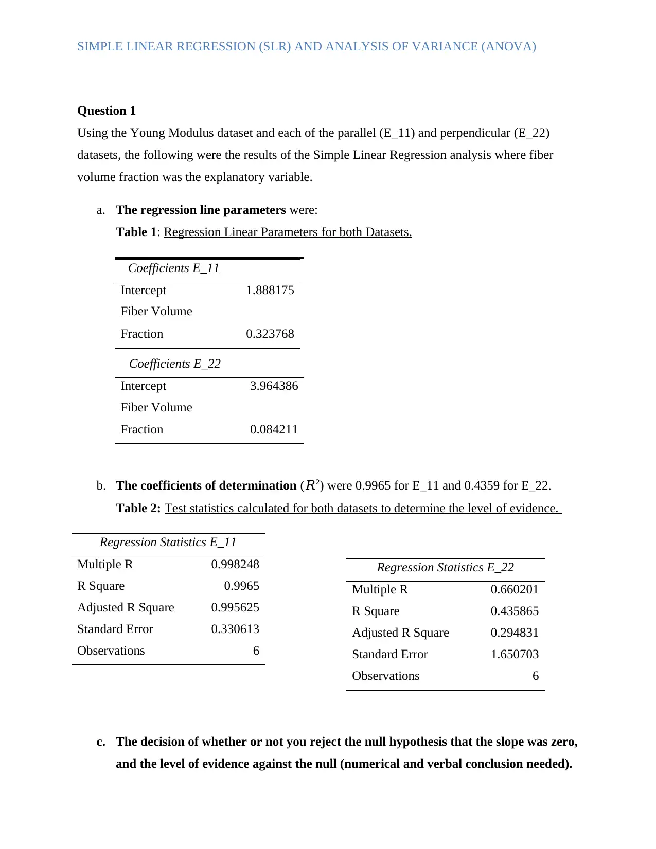
a. The regression line parameters were:
Table 1: Regression Linear Parameters for both Datasets.
Coefficients E_22
Intercept 3.964386
Fiber Volume
Fraction 0.084211
b. The coefficients of determination (𝑅2) were 0.9965 for E_11 and 0.4359 for E_22.
Table 2: Test statistics calculated for both datasets to determine the level of evidence.
c. The decision of whether or not you reject the null hypothesis that the slope was zero,
and the level of evidence against the null (numerical and verbal conclusion needed).
Coefficients E_11
Intercept 1.888175
Fiber Volume
Fraction 0.323768
Regression Statistics E_11
Multiple R 0.998248
R Square 0.9965
Adjusted R Square 0.995625
Standard Error 0.330613
Observations 6
Regression Statistics E_22
Multiple R 0.660201
R Square 0.435865
Adjusted R Square 0.294831
Standard Error 1.650703
Observations 6
SIMPLE LINEAR REGRESSION (SLR) AND ANALYSIS OF VARIANCE (ANOVA)
Test of hypothesis:
H0: B0=0, that is, the coefficients were equal to 0.
H1: B0 ≠ 0, otherwise.
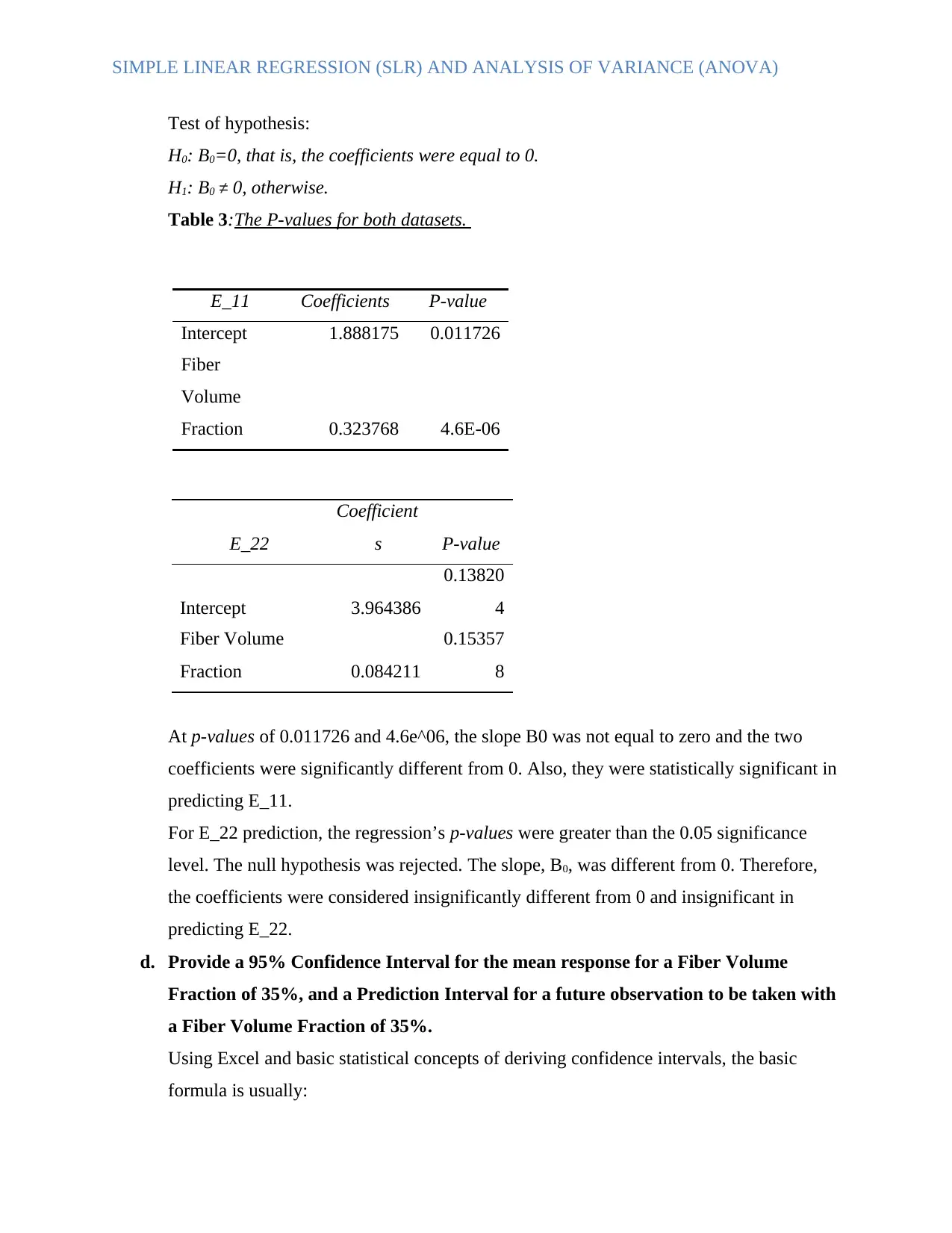
Table 3:The P-values for both datasets.
E_11 Coefficients P-value
Intercept 1.888175 0.011726
Fiber
Volume
Fraction 0.323768 4.6E-06
E_22
Coefficient
s P-value
Intercept 3.964386
0.13820
4
Fiber Volume
Fraction 0.084211
0.15357
8
At p-values of 0.011726 and 4.6e^06, the slope B0 was not equal to zero and the two
coefficients were significantly different from 0. Also, they were statistically significant in
predicting E_11.
For E_22 prediction, the regression’s p-values were greater than the 0.05 significance
level. The null hypothesis was rejected. The slope, B0, was different from 0. Therefore,
the coefficients were considered insignificantly different from 0 and insignificant in
predicting E_22.
d. Provide a 95% Confidence Interval for the mean response for a Fiber Volume
Fraction of 35%, and a Prediction Interval for a future observation to be taken with
a Fiber Volume Fraction of 35%.
Using Excel and basic statistical concepts of deriving confidence intervals, the basic
formula is usually:
⊘ This is a preview!⊘
Do you want full access?
Subscribe today to unlock all pages.

Trusted by 1+ million students worldwide
SIMPLE LINEAR REGRESSION (SLR) AND ANALYSIS OF VARIANCE (ANOVA)
Lower interval = Mean of Response(Y) – t-critical value*standard error
Upper interval = Mean of Response(Y) + t-critical value*standard error
Where the standard error is:
S.E = Standard deviation / sqrt (n)
Where n is the sample size.
The E_11 simple linear regression equation was:
E_11 = 1.888175 + 0.323768 Fiber Volume Fraction
For a Fiber Volume Fraction of 35%, the response value would be:
E_11 = 1.888175 + 0.323768*35
E_11= 1.888175 + 11.33188
E_11= 13.220055
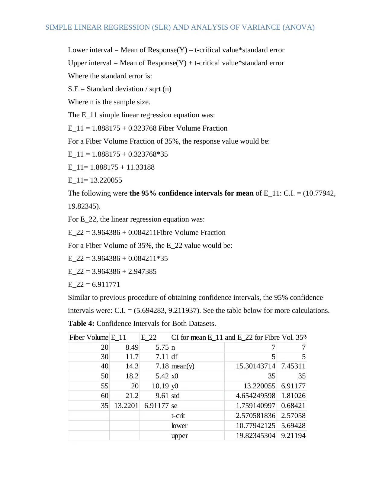
The following were the 95% confidence intervals for mean of E_11: C.I. = (10.77942,
19.82345).
For E_22, the linear regression equation was:
E_22 = 3.964386 + 0.084211Fibre Volume Fraction
For a Fiber Volume of 35%, the E_22 value would be:
E_22 = 3.964386 + 0.084211*35
E_22 = 3.964386 + 2.947385
E_22 = 6.911771
Similar to previous procedure of obtaining confidence intervals, the 95% confidence
intervals were: C.I. = (5.694283, 9.211937). See the table below for more calculations.
Table 4: Confidence Intervals for Both Datasets.
Fiber Volume FractionE_11 E_22 CI for mean E_11 and E_22 for Fibre Vol. 35%
20 8.49 5.75 n 7 7
30 11.7 7.11 df 5 5
40 14.3 7.18 mean(y) 15.30143714 7.45311
50 18.2 5.42 x0 35 35
55 20 10.19 y0 13.220055 6.91177
60 21.2 9.61 std 4.654249598 1.81026
35 13.2201 6.91177 se 1.759140997 0.68421
t-crit 2.570581836 2.57058
lower 10.77942125 5.69428
upper 19.82345304 9.21194
Paraphrase This Document
Need a fresh take? Get an instant paraphrase of this document with our AI Paraphraser
SIMPLE LINEAR REGRESSION (SLR) AND ANALYSIS OF VARIANCE (ANOVA)
Note that the new X 35% Fiber Volume was added to the initial data for new degrees of
freedom (n - 2= 5) where n was initially 6 in the original dataset. All values of mean, t-
critical, standard error and standard deviations were calculated inclusive of the acquired
X0 (35) and Y0 (depended on the regression equation).
For the prediction interval, its formula is written as:
Lower = Y0 – t-critical*standard error
Upper = Y0 + t-critical*standard error
Where the standard error is:
S.E = Syx (sqrt (1 + 1/n + (x0 – mean(x)) / SSx)
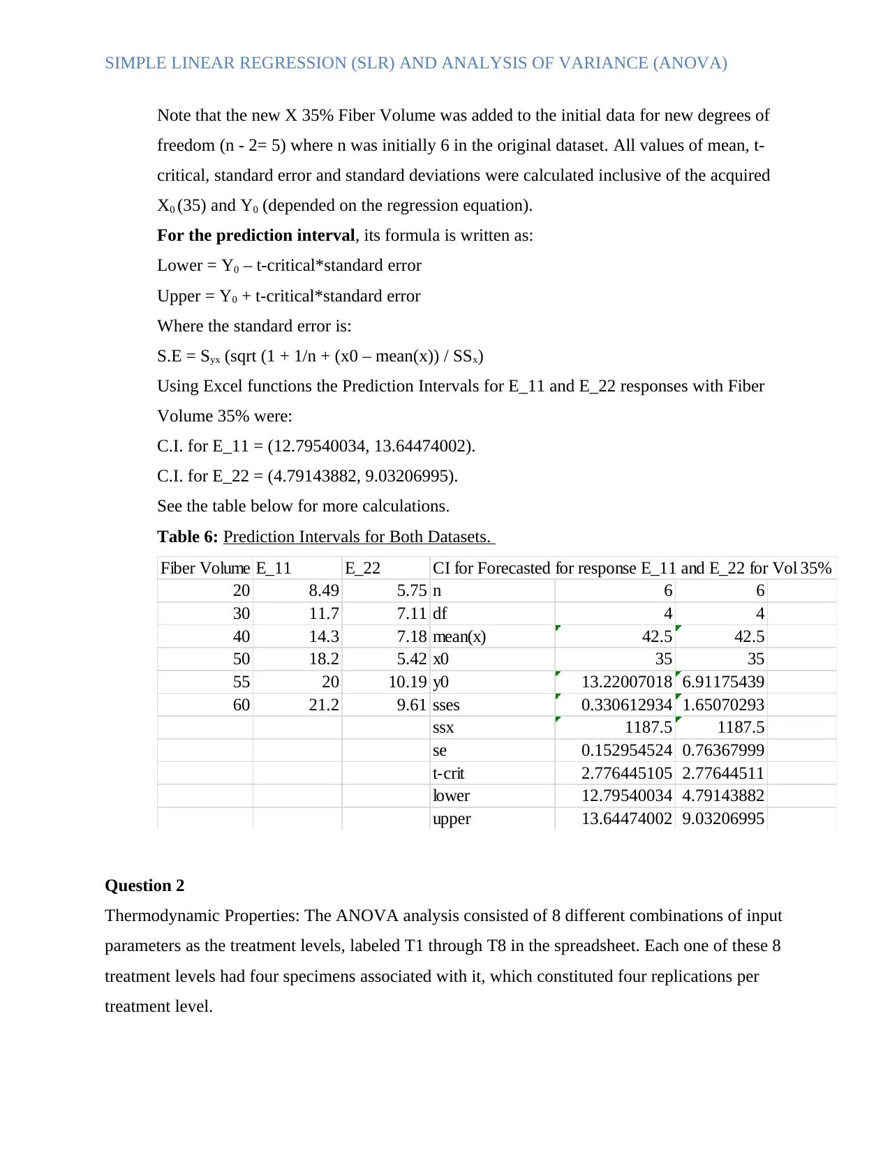
Using Excel functions the Prediction Intervals for E_11 and E_22 responses with Fiber
Volume 35% were:
C.I. for E_11 = (12.79540034, 13.64474002).
C.I. for E_22 = (4.79143882, 9.03206995).
See the table below for more calculations.
Table 6: Prediction Intervals for Both Datasets.
Fiber Volume FractionE_11 E_22 CI for Forecasted for response E_11 and E_22 for Vol 35%
20 8.49 5.75 n 6 6
30 11.7 7.11 df 4 4
40 14.3 7.18 mean(x) 42.5 42.5
50 18.2 5.42 x0 35 35
55 20 10.19 y0 13.22007018 6.91175439
60 21.2 9.61 sses 0.330612934 1.65070293
ssx 1187.5 1187.5
se 0.152954524 0.76367999
t-crit 2.776445105 2.77644511
lower 12.79540034 4.79143882
upper 13.64474002 9.03206995
Question 2
Thermodynamic Properties: The ANOVA analysis consisted of 8 different combinations of input
parameters as the treatment levels, labeled T1 through T8 in the spreadsheet. Each one of these 8
treatment levels had four specimens associated with it, which constituted four replications per
treatment level.
SIMPLE LINEAR REGRESSION (SLR) AND ANALYSIS OF VARIANCE (ANOVA)
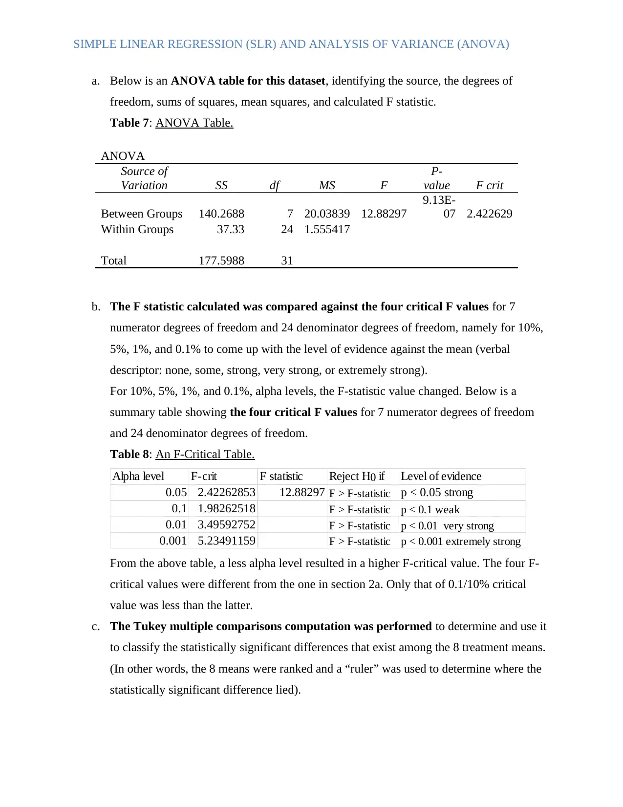
a. Below is an ANOVA table for this dataset, identifying the source, the degrees of
freedom, sums of squares, mean squares, and calculated F statistic.
Table 7: ANOVA Table.
ANOVA
Source of
Variation SS df MS F
P-
value F crit
Between Groups 140.2688 7 20.03839 12.88297
9.13E-
07 2.422629
Within Groups 37.33 24 1.555417
Total 177.5988 31
b. The F statistic calculated was compared against the four critical F values for 7
numerator degrees of freedom and 24 denominator degrees of freedom, namely for 10%,
5%, 1%, and 0.1% to come up with the level of evidence against the mean (verbal
descriptor: none, some, strong, very strong, or extremely strong).
For 10%, 5%, 1%, and 0.1%, alpha levels, the F-statistic value changed. Below is a
summary table showing the four critical F values for 7 numerator degrees of freedom
and 24 denominator degrees of freedom.
Table 8: An F-Critical Table.
Alpha level F-crit F statistic Reject H0 if Level of evidence
0.05 2.42262853 12.88297 F > F-statistic p < 0.05 strong
0.1 1.98262518 F > F-statistic p < 0.1 weak
0.01 3.49592752 F > F-statistic p < 0.01 very strong
0.001 5.23491159 F > F-statistic p < 0.001 extremely strong
From the above table, a less alpha level resulted in a higher F-critical value. The four F-
critical values were different from the one in section 2a. Only that of 0.1/10% critical
value was less than the latter.
c. The Tukey multiple comparisons computation was performed to determine and use it
to classify the statistically significant differences that exist among the 8 treatment means.
(In other words, the 8 means were ranked and a “ruler” was used to determine where the
statistically significant difference lied).
⊘ This is a preview!⊘
Do you want full access?
Subscribe today to unlock all pages.

Trusted by 1+ million students worldwide
SIMPLE LINEAR REGRESSION (SLR) AND ANALYSIS OF VARIANCE (ANOVA)
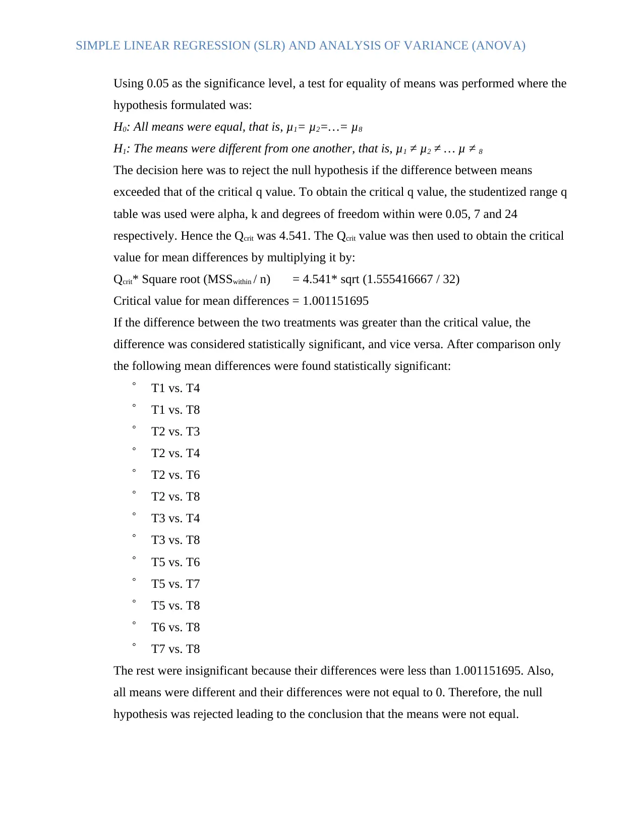
Using 0.05 as the significance level, a test for equality of means was performed where the
hypothesis formulated was:
H0: All means were equal, that is, μ1= μ2=…= μ8
H1: The means were different from one another, that is, μ1 ≠ μ2 ≠ … μ ≠ 8
The decision here was to reject the null hypothesis if the difference between means
exceeded that of the critical q value. To obtain the critical q value, the studentized range q
table was used were alpha, k and degrees of freedom within were 0.05, 7 and 24
respectively. Hence the Qcrit was 4.541. The Qcrit value was then used to obtain the critical
value for mean differences by multiplying it by:
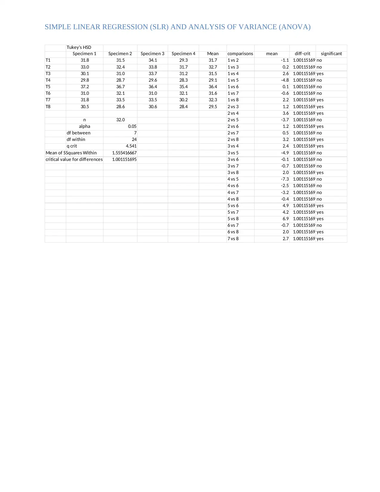
Qcrit* Square root (MSSwithin / n) = 4.541* sqrt (1.555416667 / 32)
Critical value for mean differences = 1.001151695
If the difference between the two treatments was greater than the critical value, the
difference was considered statistically significant, and vice versa. After comparison only
the following mean differences were found statistically significant:
T1 vs. T4
T1 vs. T8
T2 vs. T3
T2 vs. T4
T2 vs. T6
T2 vs. T8
T3 vs. T4
T3 vs. T8
T5 vs. T6
T5 vs. T7
T5 vs. T8
T6 vs. T8
T7 vs. T8
The rest were insignificant because their differences were less than 1.001151695. Also,
all means were different and their differences were not equal to 0. Therefore, the null
hypothesis was rejected leading to the conclusion that the means were not equal.
Paraphrase This Document
Need a fresh take? Get an instant paraphrase of this document with our AI Paraphraser
SIMPLE LINEAR REGRESSION (SLR) AND ANALYSIS OF VARIANCE (ANOVA)
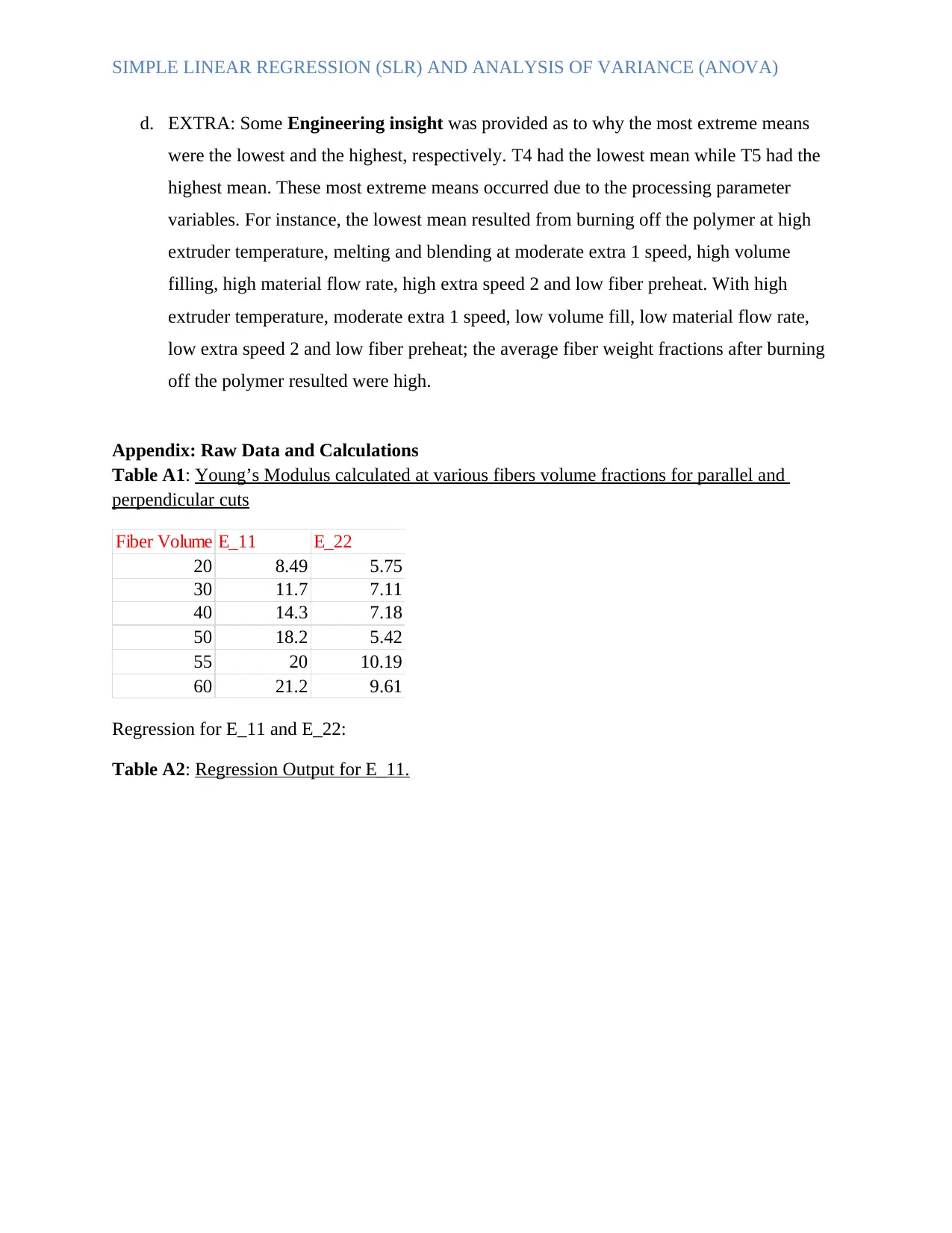
d. EXTRA: Some Engineering insight was provided as to why the most extreme means
were the lowest and the highest, respectively. T4 had the lowest mean while T5 had the
highest mean. These most extreme means occurred due to the processing parameter
variables. For instance, the lowest mean resulted from burning off the polymer at high
extruder temperature, melting and blending at moderate extra 1 speed, high volume
filling, high material flow rate, high extra speed 2 and low fiber preheat. With high
extruder temperature, moderate extra 1 speed, low volume fill, low material flow rate,
low extra speed 2 and low fiber preheat; the average fiber weight fractions after burning
off the polymer resulted were high.
Appendix: Raw Data and Calculations
Table A1: Young’s Modulus calculated at various fibers volume fractions for parallel and
perpendicular cuts
Fiber Volume FractionE_11 E_22
20 8.49 5.75
30 11.7 7.11
40 14.3 7.18
50 18.2 5.42
55 20 10.19
60 21.2 9.61
Regression for E_11 and E_22:
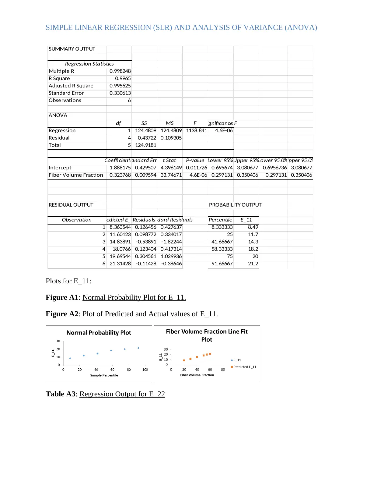
Table A2: Regression Output for E_11.
SIMPLE LINEAR REGRESSION (SLR) AND ANALYSIS OF VARIANCE (ANOVA)
SUMMARY OUTPUT
Regression Statistics
Multiple R 0.998248
R Square 0.9965
Adjusted R Square 0.995625
Standard Error 0.330613
Observations 6
ANOVA
df SS MS F Significance F
Regression 1 124.4809 124.4809 1138.841 4.6E-06
Residual 4 0.43722 0.109305
Total 5 124.9181
CoefficientsStandard Error t Stat P-value Lower 95%Upper 95%Lower 95.0%Upper 95.0%
Intercept 1.888175 0.429507 4.396149 0.011726 0.695674 3.080677 0.6956736 3.080677
Fiber Volume Fraction 0.323768 0.009594 33.74671 4.6E-06 0.297131 0.350406 0.297131 0.350406
RESIDUAL OUTPUT PROBABILITY OUTPUT
Observation Predicted E_11ResidualsStandard Residuals Percentile E_11
1 8.363544 0.126456 0.427637 8.333333 8.49
2 11.60123 0.098772 0.334017 25 11.7
3 14.83891 -0.53891 -1.82244 41.66667 14.3
4 18.0766 0.123404 0.417314 58.33333 18.2
5 19.69544 0.304561 1.029936 75 20
6 21.31428 -0.11428 -0.38646 91.66667 21.2
Plots for E_11:
Figure A1: Normal Probability Plot for E_11.
Figure A2: Plot of Predicted and Actual values of E_11.
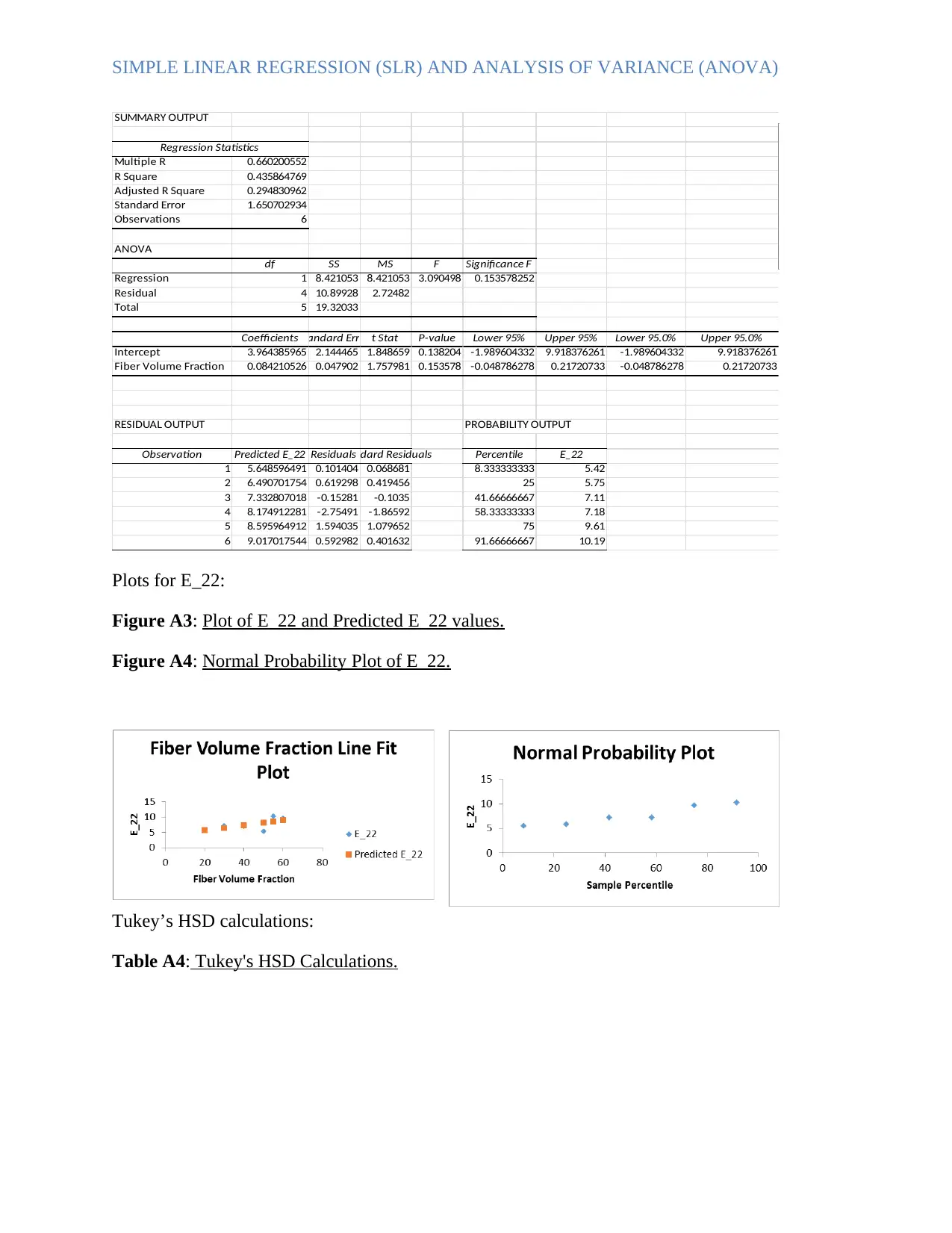
Table A3: Regression Output for E_22
⊘ This is a preview!⊘
Do you want full access?
Subscribe today to unlock all pages.

Trusted by 1+ million students worldwide
SIMPLE LINEAR REGRESSION (SLR) AND ANALYSIS OF VARIANCE (ANOVA)
SUMMARY OUTPUT
Regression Statistics
Multiple R 0.660200552
R Square 0.435864769
Adjusted R Square 0.294830962
Standard Error 1.650702934
Observations 6
ANOVA
df SS MS F Significance F
Regression 1 8.421053 8.421053 3.090498 0.153578252
Residual 4 10.89928 2.72482
Total 5 19.32033
CoefficientsStandard Error t Stat P-value Lower 95% Upper 95% Lower 95.0% Upper 95.0%
Intercept 3.964385965 2.144465 1.848659 0.138204 -1.989604332 9.918376261 -1.989604332 9.918376261
Fiber Volume Fraction 0.084210526 0.047902 1.757981 0.153578 -0.048786278 0.21720733 -0.048786278 0.21720733
RESIDUAL OUTPUT PROBABILITY OUTPUT
Observation Predicted E_22 ResidualsStandard Residuals Percentile E_22
1 5.648596491 0.101404 0.068681 8.333333333 5.42
2 6.490701754 0.619298 0.419456 25 5.75
3 7.332807018 -0.15281 -0.1035 41.66666667 7.11
4 8.174912281 -2.75491 -1.86592 58.33333333 7.18
5 8.595964912 1.594035 1.079652 75 9.61
6 9.017017544 0.592982 0.401632 91.66666667 10.19
Plots for E_22:
Figure A3: Plot of E_22 and Predicted E_22 values.
Figure A4: Normal Probability Plot of E_22.
Tukey’s HSD calculations:
Table A4: Tukey's HSD Calculations.
Paraphrase This Document
Need a fresh take? Get an instant paraphrase of this document with our AI Paraphraser
SIMPLE LINEAR REGRESSION (SLR) AND ANALYSIS OF VARIANCE (ANOVA)
Tukey's HSD
Specimen 1 Specimen 2 Specimen 3 Specimen 4 Mean comparisons mean diff-crit significant
T1 31.8 31.5 34.1 29.3 31.7 1 vs 2 -1.1 1.00115169 no
T2 33.0 32.4 33.8 31.7 32.7 1 vs 3 0.2 1.00115169 no
T3 30.1 31.0 33.7 31.2 31.5 1 vs 4 2.6 1.00115169 yes
T4 29.8 28.7 29.6 28.3 29.1 1 vs 5 -4.8 1.00115169 no
T5 37.2 36.7 36.4 35.4 36.4 1 vs 6 0.1 1.00115169 no
T6 31.0 32.1 31.0 32.1 31.6 1 vs 7 -0.6 1.00115169 no
T7 31.8 33.5 33.5 30.2 32.3 1 vs 8 2.2 1.00115169 yes
T8 30.5 28.6 30.6 28.4 29.5 2 vs 3 1.2 1.00115169 yes
2 vs 4 3.6 1.00115169 yes
n 32.0 2 vs 5 -3.7 1.00115169 no
alpha 0.05 2 vs 6 1.2 1.00115169 yes
df between 7 2 vs 7 0.5 1.00115169 no
df within 24 2 vs 8 3.2 1.00115169 yes
q crit 4.541 3 vs 4 2.4 1.00115169 yes
Mean of SSquares Within 1.555416667 3 vs 5 -4.9 1.00115169 no
critical value for differences in mean1.001151695 3 vs 6 -0.1 1.00115169 no
3 vs 7 -0.7 1.00115169 no
3 vs 8 2.0 1.00115169 yes
4 vs 5 -7.3 1.00115169 no
4 vs 6 -2.5 1.00115169 no
4 vs 7 -3.2 1.00115169 no
4 vs 8 -0.4 1.00115169 no
5 vs 6 4.9 1.00115169 yes
5 vs 7 4.2 1.00115169 yes
5 vs 8 6.9 1.00115169 yes
6 vs 7 -0.7 1.00115169 no
6 vs 8 2.0 1.00115169 yes
7 vs 8 2.7 1.00115169 yes
1 out of 11