Linear Regression Analysis: Simple vs Multiple Models

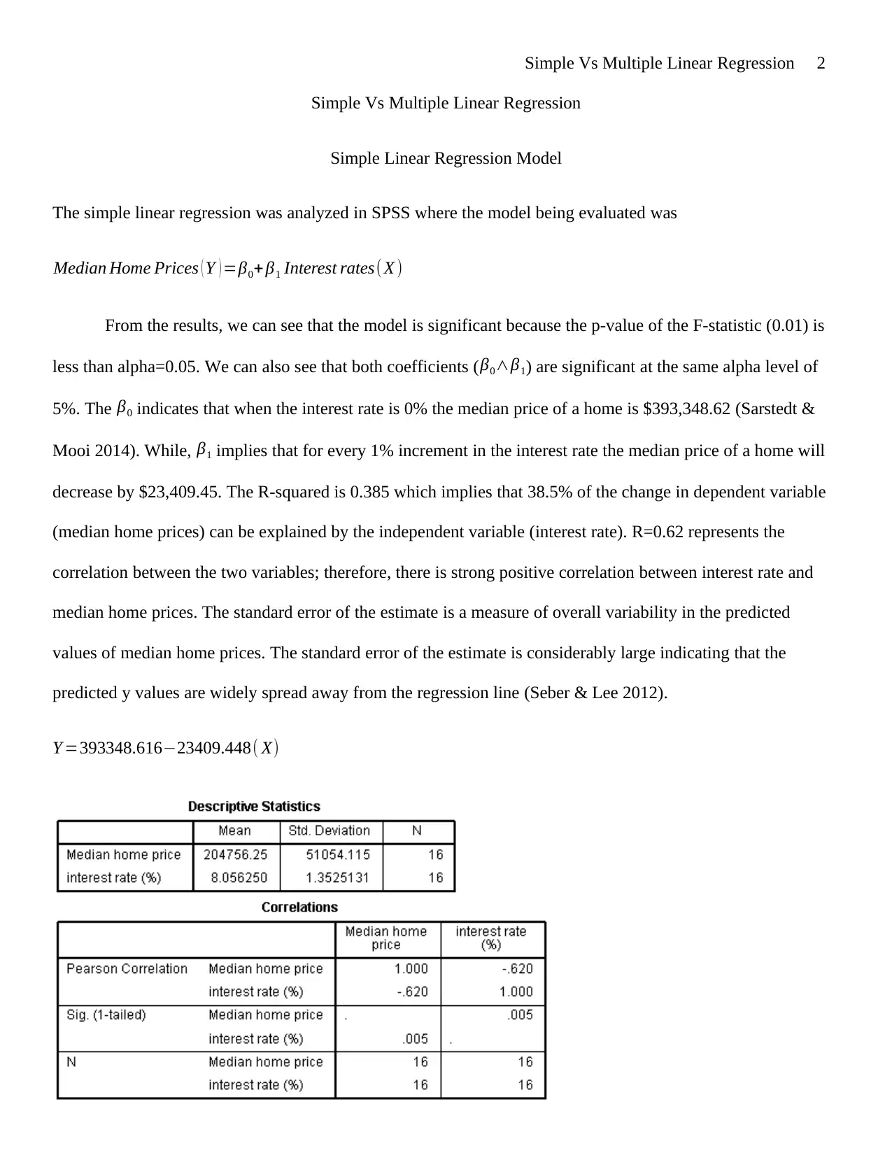
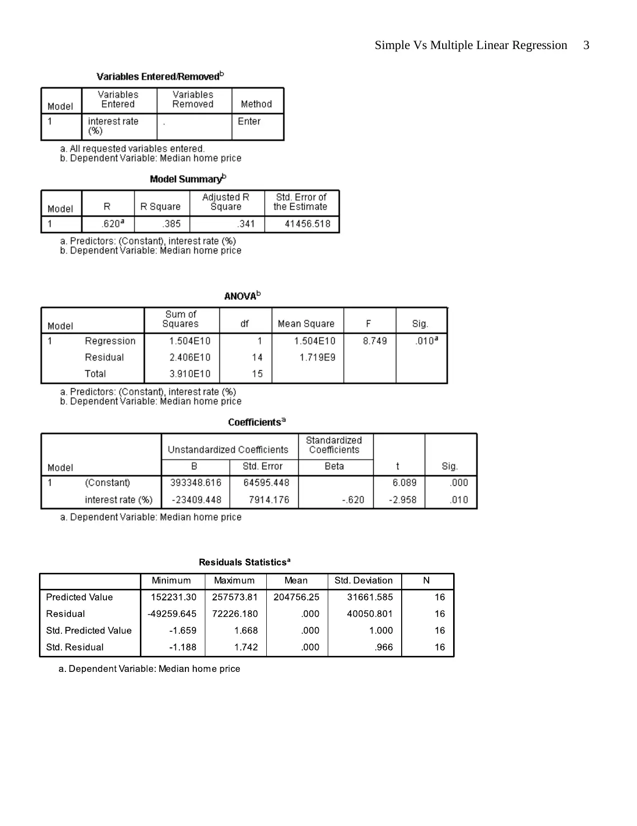
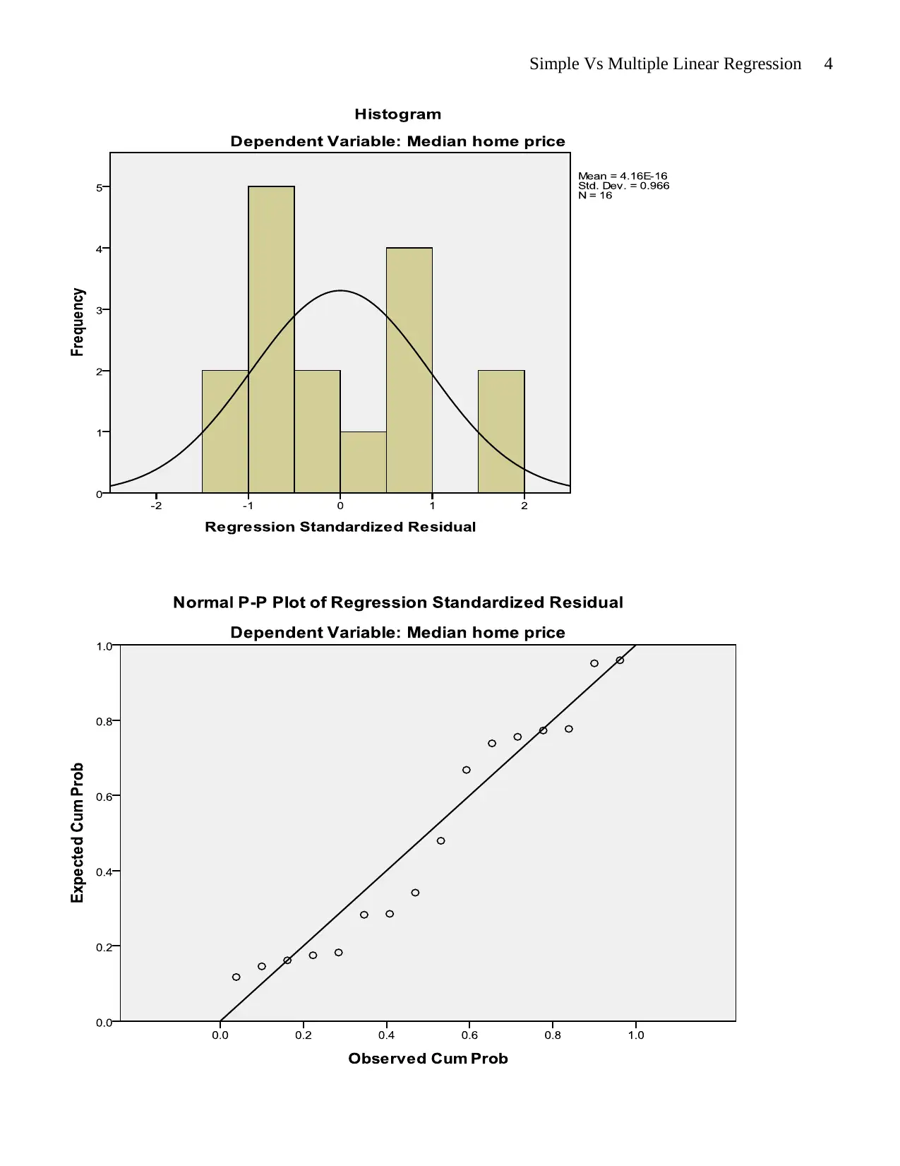
This report presents a comprehensive analysis of both simple and multiple linear regression models. The simple linear regression model examines the relationship between median home prices and interest rates, revealing a significant negative correlation. The multiple linear regression model investigates the relationship between sales and multiple independent variables, including age, HS, income, Black, Female, and price. The report interprets key statistical findings such as p-values, coefficients, R-squared, and Cronbach's Alpha to assess the significance and reliability of each model. Furthermore, the report addresses hypothesis testing, confidence intervals, and the impact of removing variables from the regression equation. The analysis includes interpretations of the coefficients and their implications on the dependent variables. The report concludes with a discussion of the limitations and strengths of each model, offering insights into the practical application of linear regression techniques.

Simple Vs Multiple Linear Regression 1
Simple Vs Multiple Linear Regression
By (Name)
The Name of the Class (Course)
Professor (Tutor)
The Name of the School (University)
The City and State where it is located
The Date

Simple Vs Multiple Linear Regression 2
Simple Vs Multiple Linear Regression
Simple Linear Regression Model
The simple linear regression was analyzed in SPSS where the model being evaluated was
Median Home Prices ( Y ) =β0+ β1 Interest rates( X )
From the results, we can see that the model is significant because the p-value of the F-statistic (0.01) is
less than alpha=0.05. We can also see that both coefficients ( β0∧β1) are significant at the same alpha level of
5%. The β0 indicates that when the interest rate is 0% the median price of a home is $393,348.62 (Sarstedt &
Mooi 2014). While, β1 implies that for every 1% increment in the interest rate the median price of a home will
decrease by $23,409.45. The R-squared is 0.385 which implies that 38.5% of the change in dependent variable
(median home prices) can be explained by the independent variable (interest rate). R=0.62 represents the
correlation between the two variables; therefore, there is strong positive correlation between interest rate and
median home prices. The standard error of the estimate is a measure of overall variability in the predicted
values of median home prices. The standard error of the estimate is considerably large indicating that the
predicted y values are widely spread away from the regression line (Seber & Lee 2012).
Y =393348.616−23409.448( X)

Simple Vs Multiple Linear Regression 3

Simple Vs Multiple Linear Regression 4

Simple Vs Multiple Linear Regression 5
Multiple Linear Regression Model
The multiple-linear regression model will be represented by the following equation
Sales ( Y ) =β0+ β1 Age ( X1 ) +β2 HS ( X2 ) + β3 Income ( X3 ) + β4 Black ( X4 ) + β5 Female ( X5 ) +β6 Price ( X6 )
We can see from the result bellow that the f-statistic for ANOVA test is significant at alpha=0.05. Out of all the
coefficients presented it is only the one associated with price that is significant at 5% alpha.

β0 indicates that when the value of all independent variables is zero sales will be−$ 15.64 million i . e . loss of $ 15.64 mil
 β1 indicates that for every 1 year increment ∈age the sales will increaseby $ 3.175million
 β2 indicates that for every unit increment ∈HS the sales will decrease by $ 0.659 million
 β3 indicates that for every $ 1 million increment ∈income the sales will increase by $ 0.021 million

Simple Vs Multiple Linear Regression 6
 β4 indicatesthat for every 1 personincrement ∈black the sales will increase by $ 0.267 million
 β5 indicates that for every 1 personincrement ∈female the sales will increase by $ 2,062 million
 β6 indicates that for every $ 1 increment ∈ price the sales will decrease by $ 2.763 million
The adjusted R-squared is 0.531 which means that 53.1% of the change in dependent variable can be explained
by the independent variables. (Sarstedt & Mooi 2014) The R of 0.767 represents the correlation between the
dependent variable and the independent variables. The correlation implies a strong positive association between
the dependent variable and the independent variables. The standard error of the estimate is small indicating that
the predicted sales for cigarettes are clustered close to the regression line (Yan 2009).
Sales ( Y ) =3.175 ( X1 )−0.659 ( X2 ) +0.021 ( X3 ) +0.267 ( X4 ) +2.062 ( X5 )−2.763 ( X6 ) −15.642

Simple Vs Multiple Linear Regression 7

Simple Vs Multiple Linear Regression 8

Simple Vs Multiple Linear Regression 9

Simple Vs Multiple Linear Regression 10
Interpreting the Cronbach’s Alpha test of reliability we see that the independent variables are not reliable in the
approximation of the dependent variable sale. The ideal Cronbach’s Alpha has to be greater than or equal to 0.7,
in this situation the Cronbach’s alpha is far below that at 0.321.
Questions in Text Book
Part (a): Test the hypothesis that the variable Female is not needed in the regression equation relating to
Sales
We will not reject the hypothesis that the variable female is not needed in the regression model above because
its p-value of 0.494 is greater than the alpha level of 0.05.

Simple Vs Multiple Linear Regression 11
Part (b): Test the hypothesis that the variables Female and HS are not needed in the above regression
equation
We will not reject the hypothesis that the variables female and HS are not needed in the regression model above
because their p-values of 0.494 and 0.134 respectively are greater than the alpha level of 0.05.
Part (c): Find the 95% confidence interval for the true regression coefficient of the variable Income
The 95% confidence interval for the coefficient of income is given as follows
Critical t=2.0096
SE=0.006
Coefficient=0.021
0.021 ± ( 2.0096 ) (0.006)
95% confidence interval (0.22206, 0.19794)
Part (d): What percentage of the variation in Sales can be accounted for when Income is removed from
the above regression equation?
When income is removed only 39.1% of the change in the dependent variable can be explained by the
remaining independent variables i.e. Price, HS, Age, Black, and Female. There is a reduction in the overall
value of adjusted R-squared this is because the effect of income on the sales of cigarettes is critical and needs to
be included in the model

Simple Vs Multiple Linear Regression 12
Part (e): The percentage of the variation in Sales can be accounted for by the three variables: Price, Age,
and Income?
When Black, Females, and HS are removed, only 42.6% of the change in the dependent variable can be
explained by the remaining independent variables i.e. Price, Age, and Income. There is a reduction in the
overall value of adjusted R-squared this is because the effect of one or more of the removed variables on the
sales of cigarettes is critical and needs to be included in the model.
Part (f): What percentage of the variation in Sales that can be accounted for by the variable Income, when
Sales is regressed on only Income?
When Black, Females, Price, HS, and Age are removed, only 13.4% of the change in the dependent variable can
be explained by the remaining independent variables i.e. income. This means that income has only 13.4% on the
overall sales recorded for cigarettes; the remaining 86.6% is caused by other factors.