Assignment on Speech Recognition Using Shallow Neural Network Classification

Running head: Speech Recognition Using Shallow Neural Network Classification
Speech Recognition Using Shallow Neural Network Classification
Name of the Student
Name of the University
Author Note

1Speech Recognition Using Shallow Neural Network Classification
Table of Contents
Introduction:...............................................................................................................................2
Problem definition:.....................................................................................................................3
Methodology:.............................................................................................................................3
Experiments and discussion:..................................................................................................5
Bayesian regularization algorithm:........................................................................................6
MATLAB code:.....................................................................................................................9
Neural network architecture view:.......................................................................................11
Network training summary:.................................................................................................11
Plot of training state:............................................................................................................12
Error histogram for test set:..................................................................................................13
ROC plot for test classes:.....................................................................................................14
Plot of confusion matrix:......................................................................................................15
Conclusion:..............................................................................................................................16
References:...............................................................................................................................17

2Speech Recognition Using Shallow Neural Network Classification
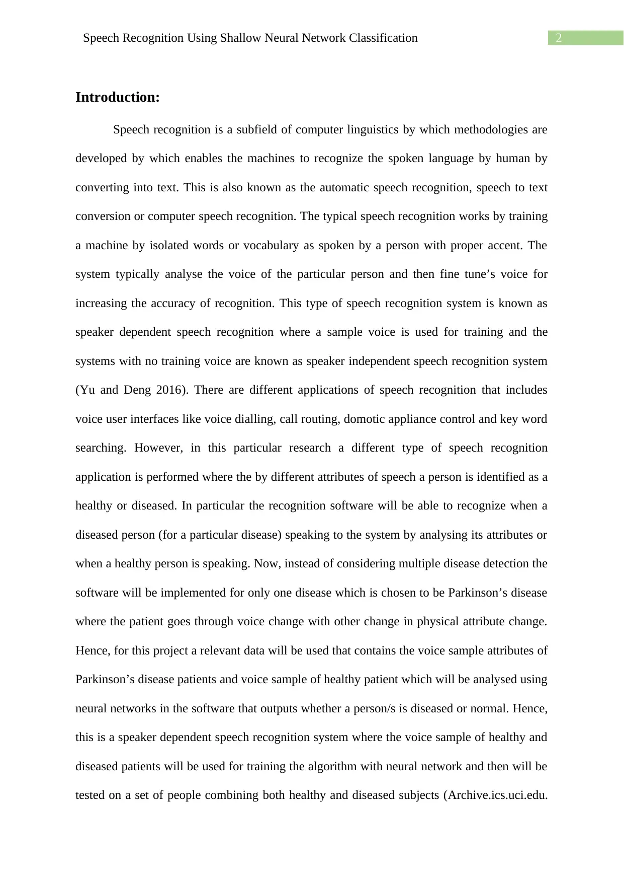
Introduction:
Speech recognition is a subfield of computer linguistics by which methodologies are
developed by which enables the machines to recognize the spoken language by human by
converting into text. This is also known as the automatic speech recognition, speech to text
conversion or computer speech recognition. The typical speech recognition works by training
a machine by isolated words or vocabulary as spoken by a person with proper accent. The
system typically analyse the voice of the particular person and then fine tune’s voice for
increasing the accuracy of recognition. This type of speech recognition system is known as
speaker dependent speech recognition where a sample voice is used for training and the
systems with no training voice are known as speaker independent speech recognition system
(Yu and Deng 2016). There are different applications of speech recognition that includes
voice user interfaces like voice dialling, call routing, domotic appliance control and key word
searching. However, in this particular research a different type of speech recognition
application is performed where the by different attributes of speech a person is identified as a
healthy or diseased. In particular the recognition software will be able to recognize when a
diseased person (for a particular disease) speaking to the system by analysing its attributes or
when a healthy person is speaking. Now, instead of considering multiple disease detection the
software will be implemented for only one disease which is chosen to be Parkinson’s disease
where the patient goes through voice change with other change in physical attribute change.
Hence, for this project a relevant data will be used that contains the voice sample attributes of
Parkinson’s disease patients and voice sample of healthy patient which will be analysed using
neural networks in the software that outputs whether a person/s is diseased or normal. Hence,
this is a speaker dependent speech recognition system where the voice sample of healthy and
diseased patients will be used for training the algorithm with neural network and then will be
tested on a set of people combining both healthy and diseased subjects (Archive.ics.uci.edu.

3Speech Recognition Using Shallow Neural Network Classification
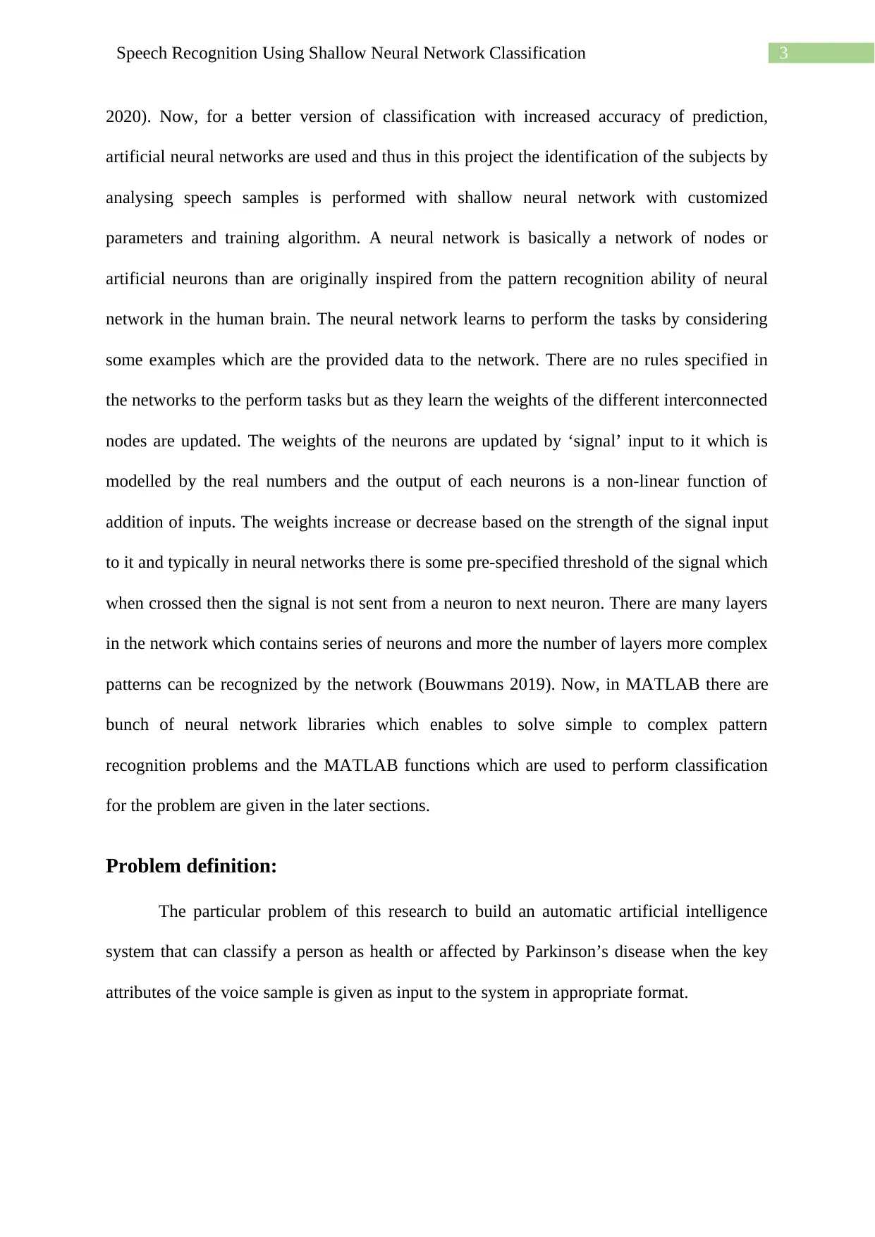
2020). Now, for a better version of classification with increased accuracy of prediction,
artificial neural networks are used and thus in this project the identification of the subjects by
analysing speech samples is performed with shallow neural network with customized
parameters and training algorithm. A neural network is basically a network of nodes or
artificial neurons than are originally inspired from the pattern recognition ability of neural
network in the human brain. The neural network learns to perform the tasks by considering
some examples which are the provided data to the network. There are no rules specified in
the networks to the perform tasks but as they learn the weights of the different interconnected
nodes are updated. The weights of the neurons are updated by ‘signal’ input to it which is
modelled by the real numbers and the output of each neurons is a non-linear function of
addition of inputs. The weights increase or decrease based on the strength of the signal input
to it and typically in neural networks there is some pre-specified threshold of the signal which
when crossed then the signal is not sent from a neuron to next neuron. There are many layers
in the network which contains series of neurons and more the number of layers more complex
patterns can be recognized by the network (Bouwmans 2019). Now, in MATLAB there are
bunch of neural network libraries which enables to solve simple to complex pattern
recognition problems and the MATLAB functions which are used to perform classification
for the problem are given in the later sections.
Problem definition:
The particular problem of this research to build an automatic artificial intelligence
system that can classify a person as health or affected by Parkinson’s disease when the key
attributes of the voice sample is given as input to the system in appropriate format.

4Speech Recognition Using Shallow Neural Network Classification
Methodology:
At first the entire dataset containing training and testing data are loaded in a
programming software. The programming software chosen for this project is MATLAB as
this has many inbuilt libraries and functions for neural networks and artificial intelligence
which are needed for training and testing with the chosen Parkinson’s data. At first the
dataset will be pre-processed to remove any missing or wrong instances and then binary class
variable will be divided in two column such that MATLAB inbuilt training functions can be
applied on the data (Gim et al. 2020). The dataset is already divided in train and test and
hence there is no need to specify the training, testing and validation ratio. The Parkinson’s
Disease speech training dataset has a total of 29 variables where variable 29 corresponds to
the class variable that has value either 1 (PD patient) or 0 (healthy patient) and the test data
set has 28 variables where variable 28 is the class variable. The additional variable in training
dataset is the UPDRS score as calculated by medical practitioner for different patients. This
variable is not used in classification as this is not available in the test set and thus the neural
networks cannot be evaluated on the test set based on this variable.
Variable information for training data:
1st column: id number of subject
2nd to 27: features of voice.
28th column: UPDRS score
29th column: information of class (1 = PD, 0 = healthy)
Test data file variable information:
1st column: id number of subject
2nd to 27th column: features of voice

5Speech Recognition Using Shallow Neural Network Classification
28th column: information of class (1 = PD, 0 = healthy)
The features of the voices has several categories containing the measures of central
tendencies and dispersions of pitch, Jitters and shimmers of the voices and other properties
that are given in details in the UCI machine learning site (Archive.ics.uci.edu. 2020).
The test data voice samples are also used for validation purpose. Now, the accuracy of
the test or validation results depends on initial weights of neurons of the neural network and
the bias vectors and thus different values of weight and bias vector should be tried in a trial
and error method until desired accuracy class detection is achieved. Also, the precision
results can be increased by increasing number of hidden layers in the network and/or training
vectors.
Now, sometimes the results are not improved by much even after trying with different
initial weights, large hidden layers and training vector. In that case it is required to apply a
different algorithm by analysing the data and the test results. The default training algorithm
of neural network is the scaled conjugate gradient algorithm. Hence, if desired accuracy of
classification is not achieved by the algorithm then a different algorithm must be tried. The
other built in algorithms that are provided by MATLAB are Levenberg-Marquardt, Bayesian
Regularization, BFGS Quasi-Newton, Resilient Backpropagation, Conjugate Gradient with
Powell/Beale Restarts, Fletcher-Powell Conjugate Gradient, Polak-Ribiére Conjugate
Gradient, One Step Secant, Variable Learning Rate Gradient Descent and Gradient Descent
algorithm (CÖMERT and Kocamaz 2017). These large variety of algorithms ensures the
accuracy of results for a wide variety of data type.
Experiments and discussion:
Now, many testing of the initial neural network is performed in sequence to improve
the performance on test case. The performance function is chosen to be mean square error

6Speech Recognition Using Shallow Neural Network Classification
which is the average of squared difference between predicted class and original target class.
In the test case all the instances belong from PD patients and hence target class is always 1.
The optimum performance is achieved with Bayesian Regularization back-propagation
method after trying all the algorithms as specified in the methodology section. Now, the
hidden layers in the network is considered enough large equal to 50 which is sufficient to
reduce approximation error produced by small number of function evaluation. Unlike other
neural network classification method, in this problem two separate data sets are used for
training and testing to confirm the applicability of classification on untrained data. Hence, the
train ratio in network training is set to 1 with validation and test ratio as 0. The final chosen
algorithm after trying different back propagation, gradient descent and conjugate gradient
algorithms the final algorithm is chosen to be Bayesian Regularization which is specified
‘trainbr’ in network parameters in MATLAB.
Bayesian regularization algorithm:
Bayesian regularized ANN are more efficient than the normal back-propagation nets and thus
the need of lengthy cross-validation can be reduced by this method. Bayesian regularization
in mathematical terms is a process by which nonlinear regression is transformed into a well
formulated problem that can be represented by ridge regression. The main advantage of the
Bayesian regularization is that through this robust models are obtained and the validation
process which takes about O(N^2) time complexity is unnecessary for this algorithm. This
type of neural networks provide solution to a various number of problem in QSAR modelling
like model choice, robustness choice, validation set choice, size of validation effort and
optimal network architecture. The overtraining in this method is very difficult as an objective
Bayesian criterion is required to stop the training (Kayri 2016). The over fitting to the data is
also quite unlikely as ‘trainbr’ calculates and then trains on a wide variety of network
parameters and weights of each node that eliminates the nodes which are not relevant. The

7Speech Recognition Using Shallow Neural Network Classification
effective number of nodes or neurons are generally very small compared to the total number
of weights in a complete back-propagation neural network. With ‘trainbr’ the ARD
(automatic relevance determination scheme) can be applied for estimating the relevance of
each input variable. This ARD method helps to filter out the irrelevant or highly correlated
variables (leading to auto-correlation) showing up only the most important variable for
modelling the network (Kayabasi et al. 2017). The ‘trainbr’ algorithm can train any type of
network in which input, weights and transfer function are differentiable. Through BR method
either the mean squared error or the sum of square error are minimized and hence the
performance function for this method cannot be cross-entropy, instead, MSE or SSE is used.
In BR method the linear combination is also modified in way such that after training good
generalization qualities of the network can be observed. The BR algorithm is basically an
extended version of the Levenberg-Marquardt algorithm where the back-propagation is used
for calculating the Jacobian of the performance corresponding to bias variables X and the
weights. In mathematical terms the BR algorithm can be defined as follows
F = objective function
M = weights of neural network
e = error in modelling
w = net weight
D = Input-output combination of dataset
H = Hessian of the objective function calculated using Jacobian
γ= paramter of regularization
The objective function which is to be minimized given by the following equation

8Speech Recognition Using Shallow Neural Network Classification
Min, F = γ ∑
j =1
M
w j
2+(1−γ )∑
i =1
N
ei
2
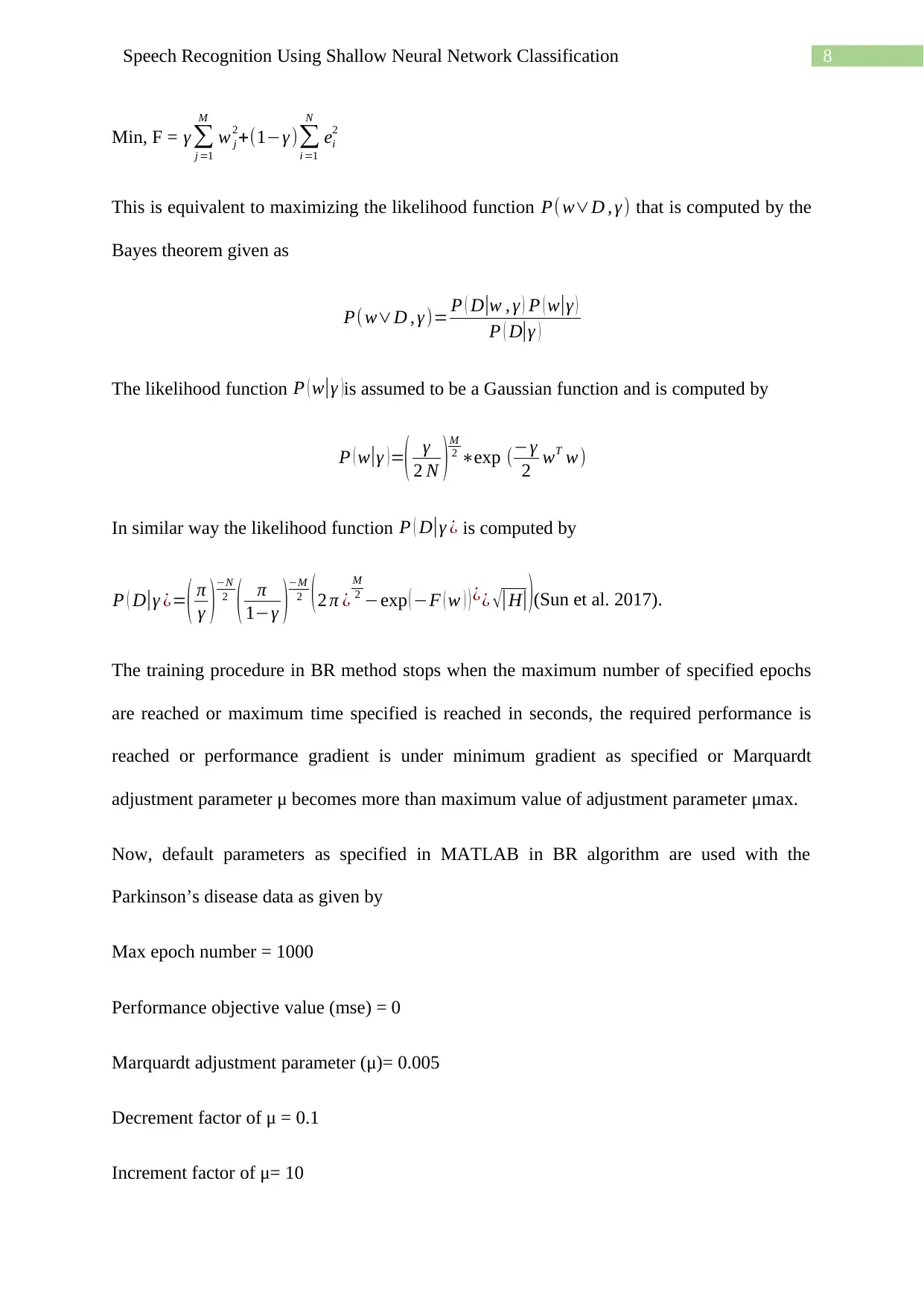
This is equivalent to maximizing the likelihood function P( w∨D , γ ) that is computed by the
Bayes theorem given as
P( w∨D , γ )= P ( D|w , γ ) P ( w|γ )
P ( D|γ )
The likelihood function P ( w|γ )is assumed to be a Gaussian function and is computed by
P ( w|γ ) =( γ
2 N ) M
2 ∗exp (−γ
2 wT w)
In similar way the likelihood function P ( D|γ ¿ is computed by
P ( D|γ ¿=( π
γ ) −N
2
( π
1−γ )
−M
2 ( 2 π ¿
M
2 −exp ( −F ( w ) ) ¿¿ √| H|)(Sun et al. 2017).
The training procedure in BR method stops when the maximum number of specified epochs
are reached or maximum time specified is reached in seconds, the required performance is
reached or performance gradient is under minimum gradient as specified or Marquardt
adjustment parameter μ becomes more than maximum value of adjustment parameter μmax.
Now, default parameters as specified in MATLAB in BR algorithm are used with the
Parkinson’s disease data as given by
Max epoch number = 1000
Performance objective value (mse) = 0
Marquardt adjustment parameter (μ)= 0.005
Decrement factor of μ = 0.1
Increment factor of μ= 10

9Speech Recognition Using Shallow Neural Network Classification
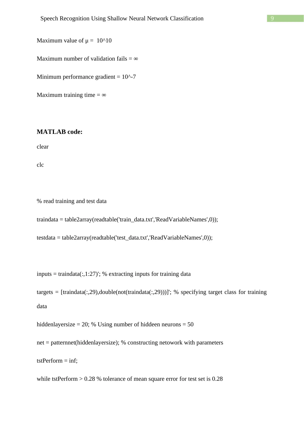
Maximum value of μ = 10^10
Maximum number of validation fails = ∞
Minimum performance gradient = 10^-7
Maximum training time = ∞
MATLAB code:
clear
clc
% read training and test data
traindata = table2array(readtable('train_data.txt','ReadVariableNames',0));
testdata = table2array(readtable('test_data.txt','ReadVariableNames',0));
inputs = traindata(:,1:27)'; % extracting inputs for training data
targets = [traindata(:,29),double(not(traindata(:,29)))]'; % specifying target class for training
data
hiddenlayersize = 20; % Using number of hiddeen neurons = 50
net = patternnet(hiddenlayersize); % constructing netowork with parameters
tstPerform = inf;
while tstPerform > 0.28 % tolerance of mean square error for test set is 0.28

10Speech Recognition Using Shallow Neural Network Classification
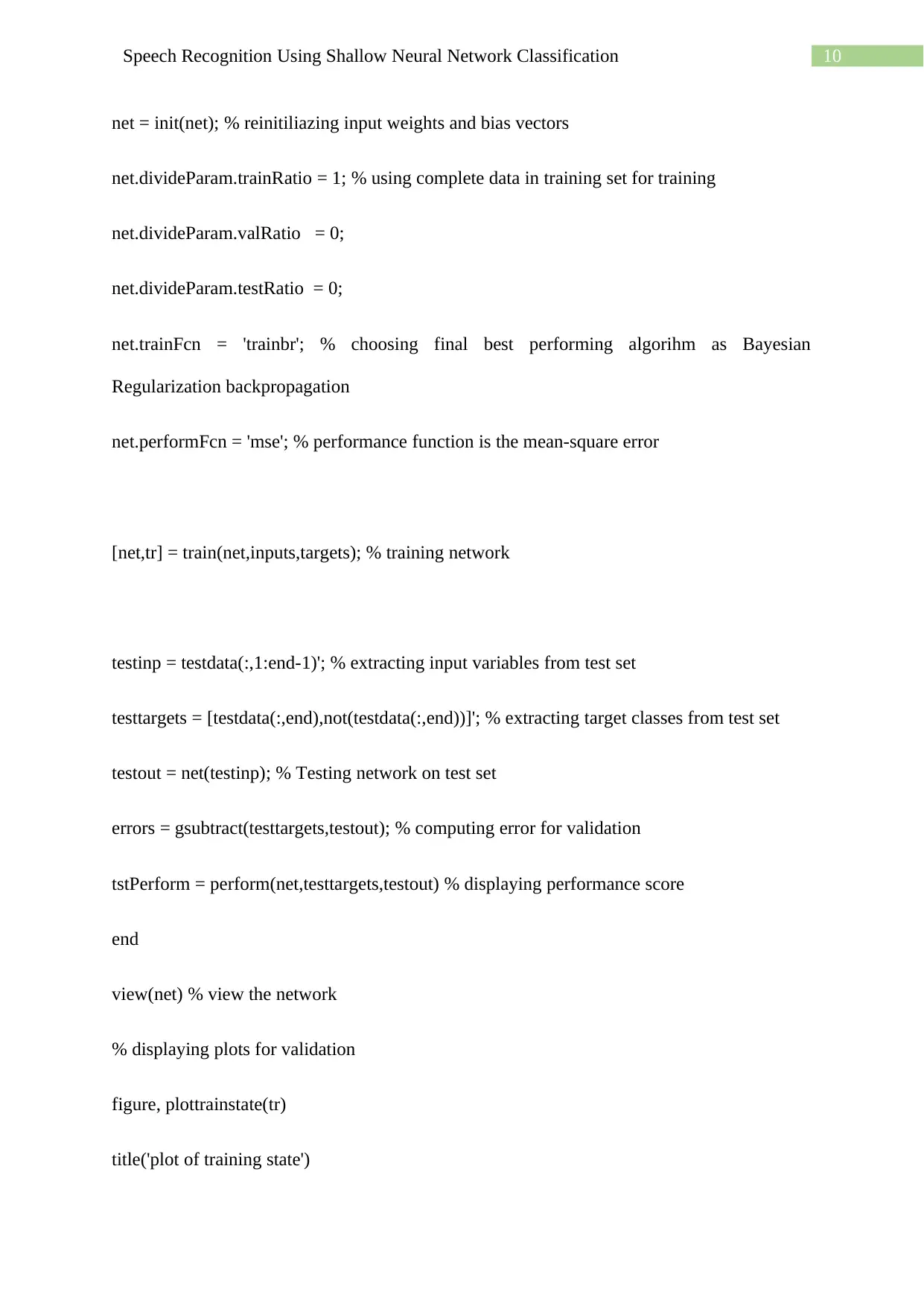
net = init(net); % reinitiliazing input weights and bias vectors
net.divideParam.trainRatio = 1; % using complete data in training set for training
net.divideParam.valRatio = 0;
net.divideParam.testRatio = 0;
net.trainFcn = 'trainbr'; % choosing final best performing algorihm as Bayesian
Regularization backpropagation
net.performFcn = 'mse'; % performance function is the mean-square error
[net,tr] = train(net,inputs,targets); % training network
testinp = testdata(:,1:end-1)'; % extracting input variables from test set
testtargets = [testdata(:,end),not(testdata(:,end))]'; % extracting target classes from test set
testout = net(testinp); % Testing network on test set
errors = gsubtract(testtargets,testout); % computing error for validation
tstPerform = perform(net,testtargets,testout) % displaying performance score
end
view(net) % view the network
% displaying plots for validation
figure, plottrainstate(tr)
title('plot of training state')

11Speech Recognition Using Shallow Neural Network Classification
figure, ploterrhist(errors)
title('Error plot for test set')
figure, plotroc(testtargets,testout)
title('Receiver operating Characteristics for test set')
figure, plotconfusion(testtargets,testout)
title('Confusion matrix plot for test set')
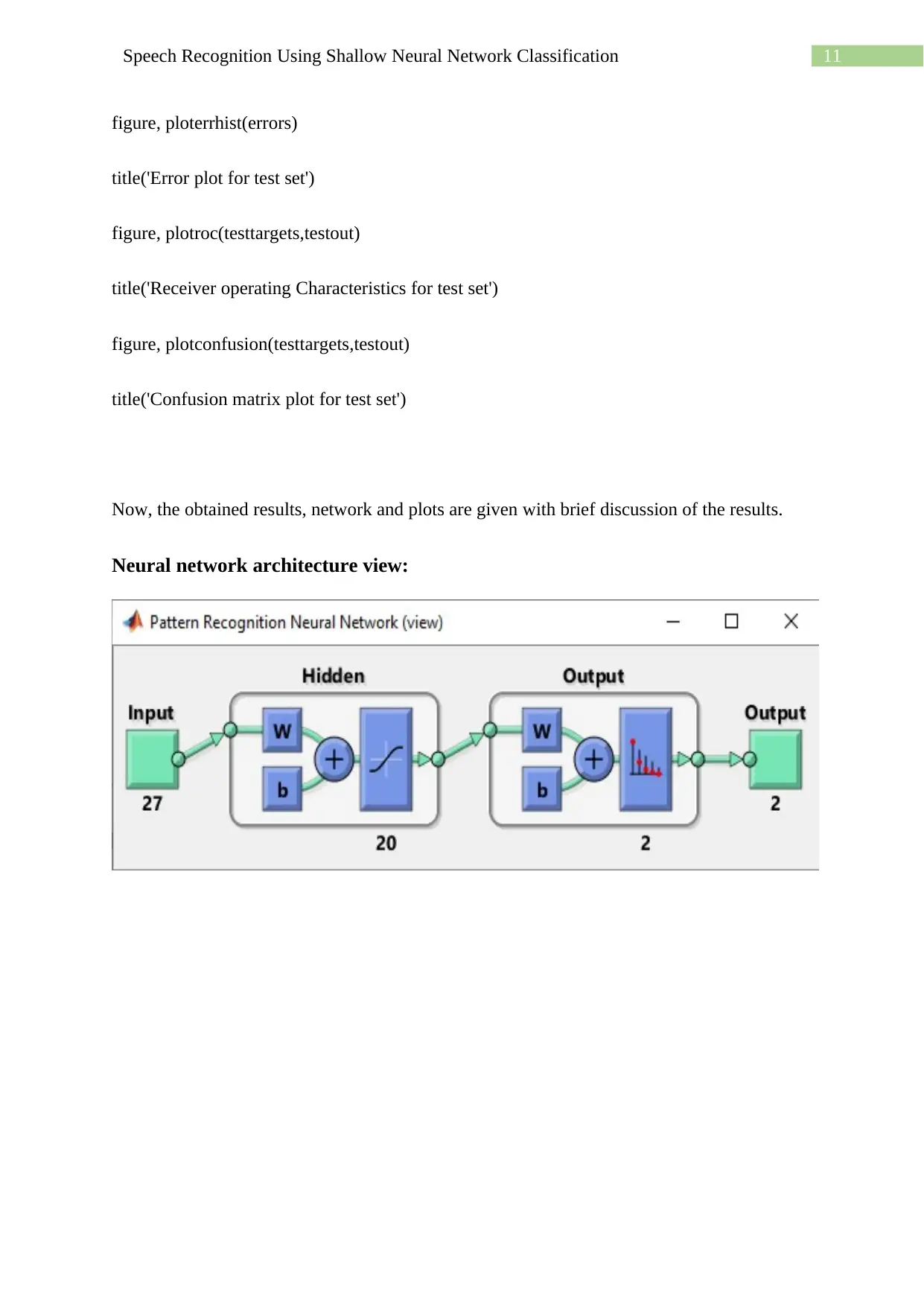
Now, the obtained results, network and plots are given with brief discussion of the results.
Neural network architecture view:

12Speech Recognition Using Shallow Neural Network Classification
Network training summary:
As it can be seen from the training summary results that the algorithm is stopped because the
performance gradient (7*10^-8) is less than the minimum specified gradient of 10^-7. At this
iteration the performance MSE value achieved is 9.85*10^-10 which is very low and thus
there is negligible amount of error in fitting with the actual class values. The final μ is found
to be 50 which is less than maximum specified μ in the algorithm. The effective number of
parameters as found by the algorithm is 59.5 at the last iteration which was initially as 602.
The algorithm stops after 43 iterations taking about 5 seconds and hence the algorithm
performs classification in an efficient way.

13Speech Recognition Using Shallow Neural Network Classification
Plot of training state:
10-5
100
gradient Gradient = 7.1113e-08, at epoch 43
100
mu
Mu = 50, at epoch 43
0
500
gamk
Num Parameters = 59.4609, at epoch 43
102
ssX
Sum Squared Param = 184.0055, at epoch 43
0 5 10 15 20 25 30 35 40
43 Epochs
-1
0
1
val fail
plot of training state
The plot of the training state shows that the gradient naturally decreases with number of
iterations and an increment of μ is observed, however, towards the end it can be seen that μ
settles at the end which indicates stability in the solution. The effective parameters from the
data set are found to be approximately 59.5 at the end of iteration and the sum of square
parameter is 184 at 43rd iteration.
The validation with the test set is obtained with the following plots.

14Speech Recognition Using Shallow Neural Network Classification
Error histogram for test set:
0
20
40
60
80
100
120
140
160
Instances
Error plot for test set
-0.95
-0.85
-0.75
-0.65
-0.55
-0.45
-0.35
-0.25
-0.15
-0.05
0.05
0.15
0.25
0.35
0.45
0.55
0.65
0.75
0.85
0.95
Errors
Zero Error
The error histogram for test set shows that the number of instances with error are large when
the error is low which shows good prediction of accurate classes by the algorithm. However,
a significant number of instances are observed towards both end of error histogram that
contains large error value, indicating a significant amount of classes are wrongly interpreted
by the algorithm (Pan et al. 2020).

15Speech Recognition Using Shallow Neural Network Classification
ROC plot for test classes:
The receiver operating curve shows one of class has curve of one class is hugged at the
topmost left and curve of other curve is hugged the bottom right. This indicates the neural
network is able to predict accurately one class however, the other class values are completely
wrongly evaluated. This is because the quality of classification is better when the classes are
hugging the top left corner and worse when classes are away from top left (Carter et al.
2016). The behaviour is expected because in the test set there is no 0 class in the target
variable, however, in the training set there are significant number of 0 class in target variable
and hence the network is trained in such a way to interpret some classes as 0 or not always
classify as 1.

16Speech Recognition Using Shallow Neural Network Classification
Plot of confusion matrix:
1
2
Target Class
1
2
Output Class
Confusion matrix plot for test set
123
73.2%
45
26.8%
73.2%
26.8%
0
0.0%
0
0.0%
NaN%
NaN%
100%
0.0%
0.0%
100%
73.2%
26.8%
The confusion matrix of the test set shows a detail validation of the results. The true positive
rate is found to be 73.2% for total of 123 instances and the true negative rate is 26.8% for a
total of 45 instances. Hence, the network incorrectly classified 45 instances as 0 which are
actually 1. As, there are no 0’s in the test set hence the false negative and false positive rate
are 0% each (Ruuska et al. 2018). Thus the performance of network is moderately good for

17Speech Recognition Using Shallow Neural Network Classification
identifying Parkinson’s diseased persons as over 73% of the total cases the identification is
successful.
Conclusion:
In conclusion it can be stated that the objective of this particular project is
successfully met as the artificial intelligence algorithms are successfully applied with neural
network classification technique to identify Parkinson’s diseased persons with their speech
samples. The Bayesian regularization is found to be the best performing training algorithm
for the neural network to classify subjects. Other than conventional neural network
classification a different method is used in this project where the training and test set are
completely independent which tests the ability of the network to recognize any of the voice
sample data provided in proper format. The results of classification is satisfactory as the
neural network with chosen algorithm was able to successfully identify PD patients over 73%
of cases. However, the number of incorrectly classified instances are significant it is expected
that this will reduce as some of test data is given as input to the training set in a random
manner.
The obvious limitation of the particular neural network system is that the system is
unable to perform classification when there are more than two classes of subjects in the
dataset. In that case the training and test input vectors are needed to be modified to input the
patternnet function in MATLAB. The system is not also suitable to directly process vocals of
individuals and then to classify them as diseased or healthy but some software or algorithm is
needed to be applied on the voice sample to extract the key variables as specified in the
dataset.

18Speech Recognition Using Shallow Neural Network Classification
References:
Archive.ics.uci.edu. 2020. UCI Machine Learning Repository: Parkinson Speech Dataset
With Multiple Types Of Sound Recordings Data Set. [online] Available at:
<https://archive.ics.uci.edu/ml/datasets/Parkinson+Speech+Dataset+with+
+Multiple+Types+of+Sound+Recordings#> [Accessed 19 March 2020].
Bouwmans, T., Javed, S., Sultana, M. and Jung, S.K., 2019. Deep neural network concepts
for background subtraction: A systematic review and comparative evaluation. Neural
Networks.
Carter, J.V., Pan, J., Rai, S.N. and Galandiuk, S., 2016. ROC-ing along: Evaluation and
interpretation of receiver operating characteristic curves. Surgery, 159(6), pp.1638-1645.
CÖMERT, Z. and Kocamaz, A.F., 2017. A study of artificial neural network training
algorithms for classification of cardiotocography signals. Bitlis Eren University journal of
science and technology, 7(2), pp.93-103.
Gim, Y., Jang, D.K., Sohn, D.K., Kim, H. and Ko, H.S., 2020. Three-dimensional particle
tracking velocimetry using shallow neural network for real-time analysis. Experiments in
Fluids, 61(2), pp.1-8.
Kayabasi, A., Sabanci, K., Yigit, E., Toktas, A., Yerlikaya, M. and Yildiz, B., 2017. Image
processing based ann with Bayesian regularization learning algorithm for classification of
wheat grains.

19Speech Recognition Using Shallow Neural Network Classification
Kayri, M., 2016. Predictive abilities of bayesian regularization and Levenberg–Marquardt
algorithms in artificial neural networks: a comparative empirical study on social
data. Mathematical and Computational Applications, 21(2), p.20.
Pan, Z., Gao, X., Wang, L. and Gao, E., 2020. Effective reversible data hiding using dynamic
neighboring pixels prediction based on prediction-error histogram. Multimedia Tools and
Applications, pp.1-27.
Ruuska, S., Hämäläinen, W., Kajava, S., Mughal, M., Matilainen, P. and Mononen, J., 2018.
Evaluation of the confusion matrix method in the validation of an automated system for
measuring feeding behaviour of cattle. Behavioural processes, 148, pp.56-62.
Sun, Z., Chen, Y., Li, X., Qin, X. and Wang, H., 2017. A Bayesian regularized artificial
neural network for adaptive optics forecasting. Optics Communications, 382, pp.519-527.
Yu, D. and Deng, L., 2016. AUTOMATIC SPEECH RECOGNITION. Springer london
limited.