SPSS Assessment

This document provides a detailed analysis of SPSS Assessment. It includes the impacts of Ketamine on depressed individuals and the efficiency of Ketamine treatment. The analysis is done using the SPSS software and includes descriptive statistics, ANOVA tests, and regression analysis.

SPSS Assessment
SPSS Assessment

SPSS Assessment
Query 1
a. Description
A three-week study on 93 individuals has undertaken to determine the impacts of
Ketamine on depressed individuals. In order to identify that whether or not Ketamine treatment
works over time, the method of repeated measures ANOVA is used in software application of
SPSS. There are various assumptions which repeated measures ANOVA considers which also
justifies the choice of this method. It assumes that every variable which has been selected is
independent and identically distributed. Normality of the data is also assumed as it is a
parametric test and lastly it assumes the sphericity. Besides ANOVA, a post hoc test of
Bonferroni is also selected which will further analyse that if there is a difference in Mean of
depression severity overtime then which are the pairs which has such significant difference. The
null hypothesis of such analysis states that mean of depression severity over time is equal.
b. Descriptive statistics and summary of the analyses and findings
The results which are gathered from SPSS output are in detail and are attached in
Appendix. Only the data required for analysis is represented below:
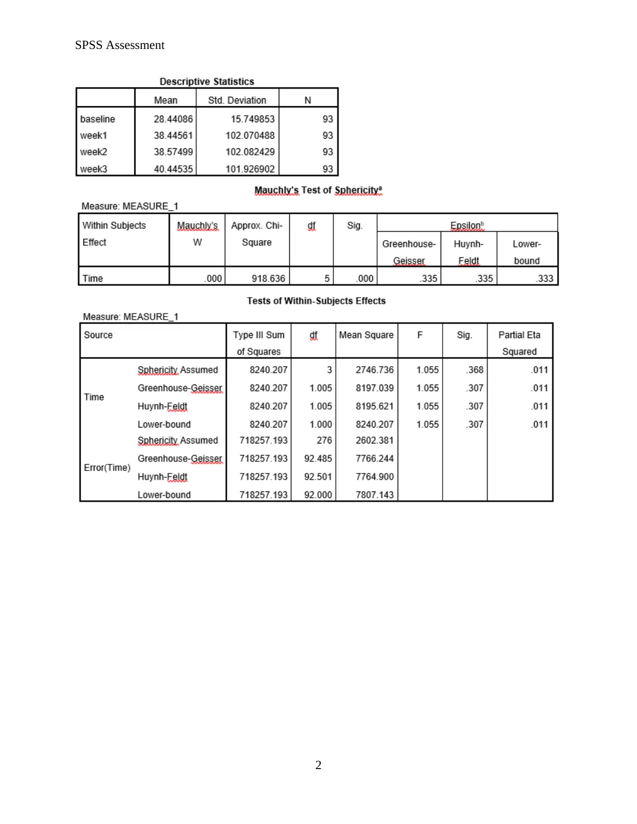
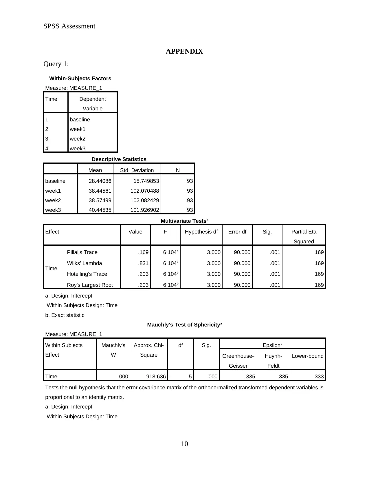
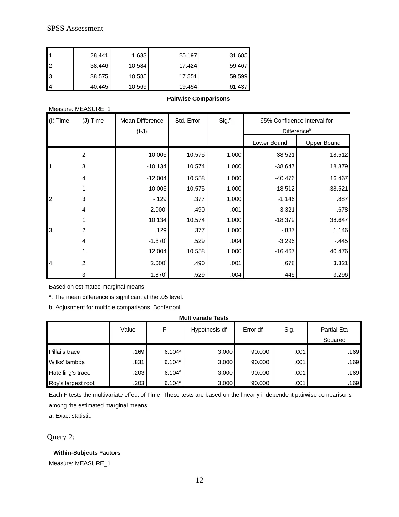
The table of descriptive statistics is showing difference mean over time as mean value for
baseline is 28.44 which increased in week 1 as 38.44, further increased in week 2 as 38.57 and
then reduced to 40.44 at the end of week 3. Descriptive statistics clearly represents that there is a
difference between the depression severity overtime but if this difference is significant or not, it
will be analysed from ANOVA test.
1

SPSS Assessment
2

SPSS Assessment
The above Mauchly’s test has the p value of .000 which is less than 0.05 implying the p
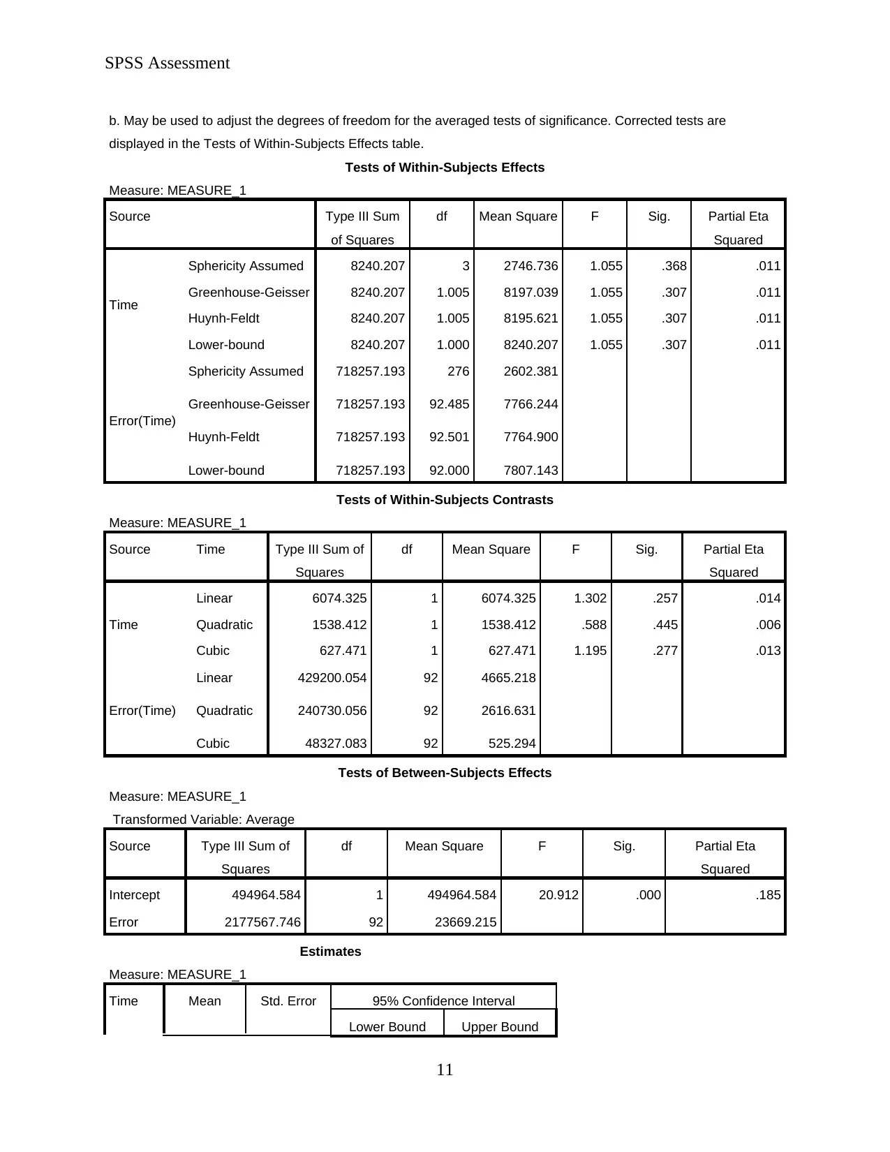
value of sphericity assumed can not be used. In the table of test of within subject effects, the p
value of Greenhouse-Geisser will be used. A repeated mesaures ANOVA determined that mean
depression severity is significant same across three time points (F(1, 92.4) = 1.05, p = .307). A
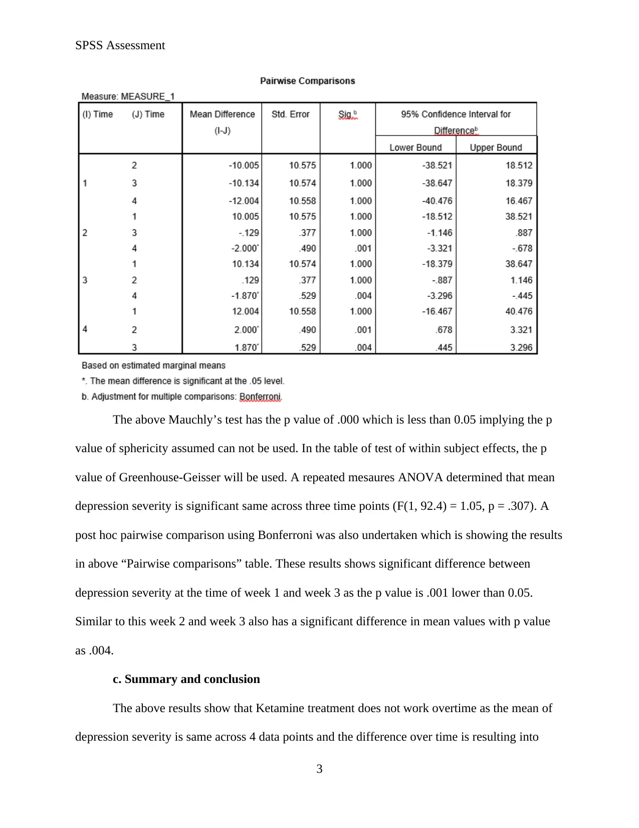
post hoc pairwise comparison using Bonferroni was also undertaken which is showing the results
in above “Pairwise comparisons” table. These results shows significant difference between
depression severity at the time of week 1 and week 3 as the p value is .001 lower than 0.05.
Similar to this week 2 and week 3 also has a significant difference in mean values with p value
as .004.
c. Summary and conclusion
The above results show that Ketamine treatment does not work overtime as the mean of
depression severity is same across 4 data points and the difference over time is resulting into
3

SPSS Assessment
increasing of such severity. This implies there is no indication that depression severity is
reducing over time by using ketamine treatment.
Query 2
a. Description
In this particular query, it is required to identify that whether Ketamine treatment works
for particular those participants which were not receiving any other treatment. For this analysis,
first the dummy variables are created. The creating of these variables are justifiable as by these
only those participants will be analysed who as “1” as their adjunct therapy representing “none”.
Further the SPSS model of repeated measures ANOVA is used similar to above query to identify
efficiency of Ketamine treatment overtime.
b. Descriptive statistics and summary of the analyses and findings
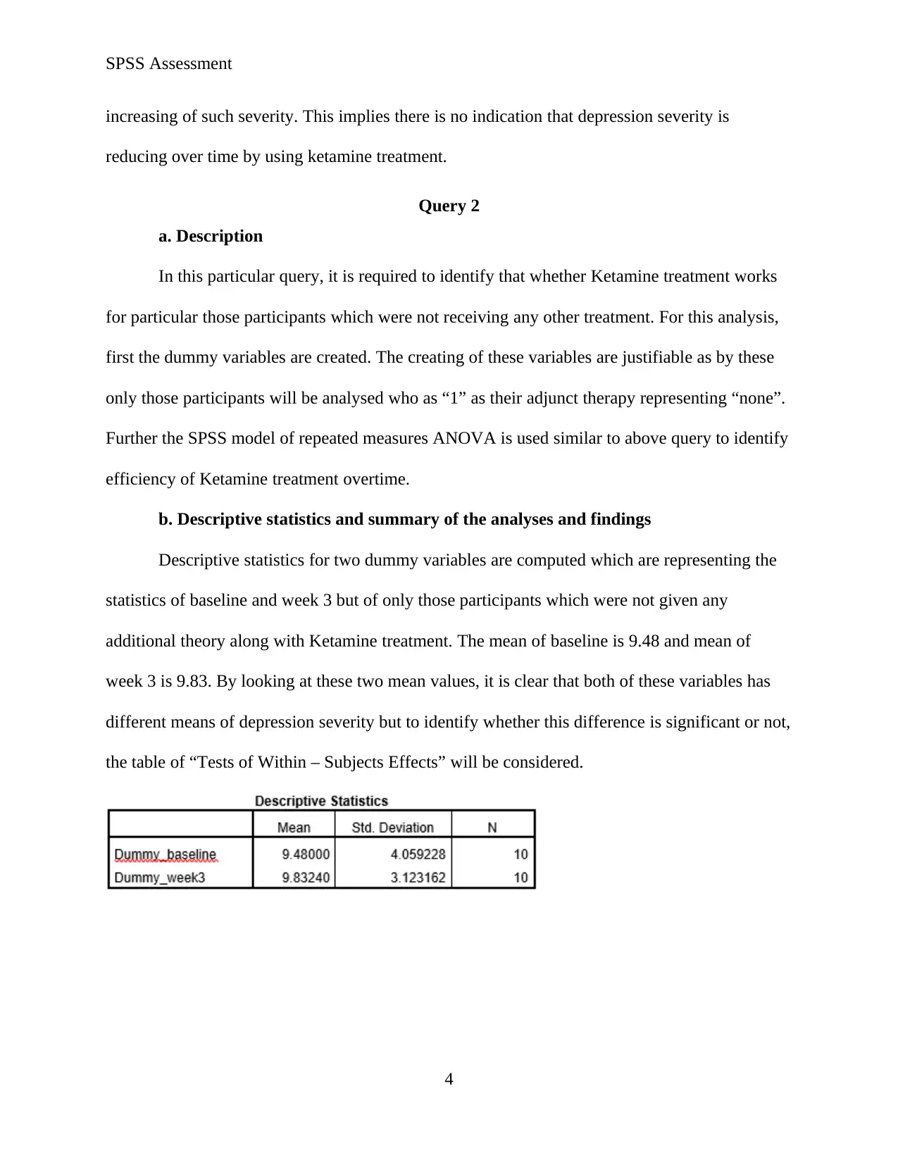
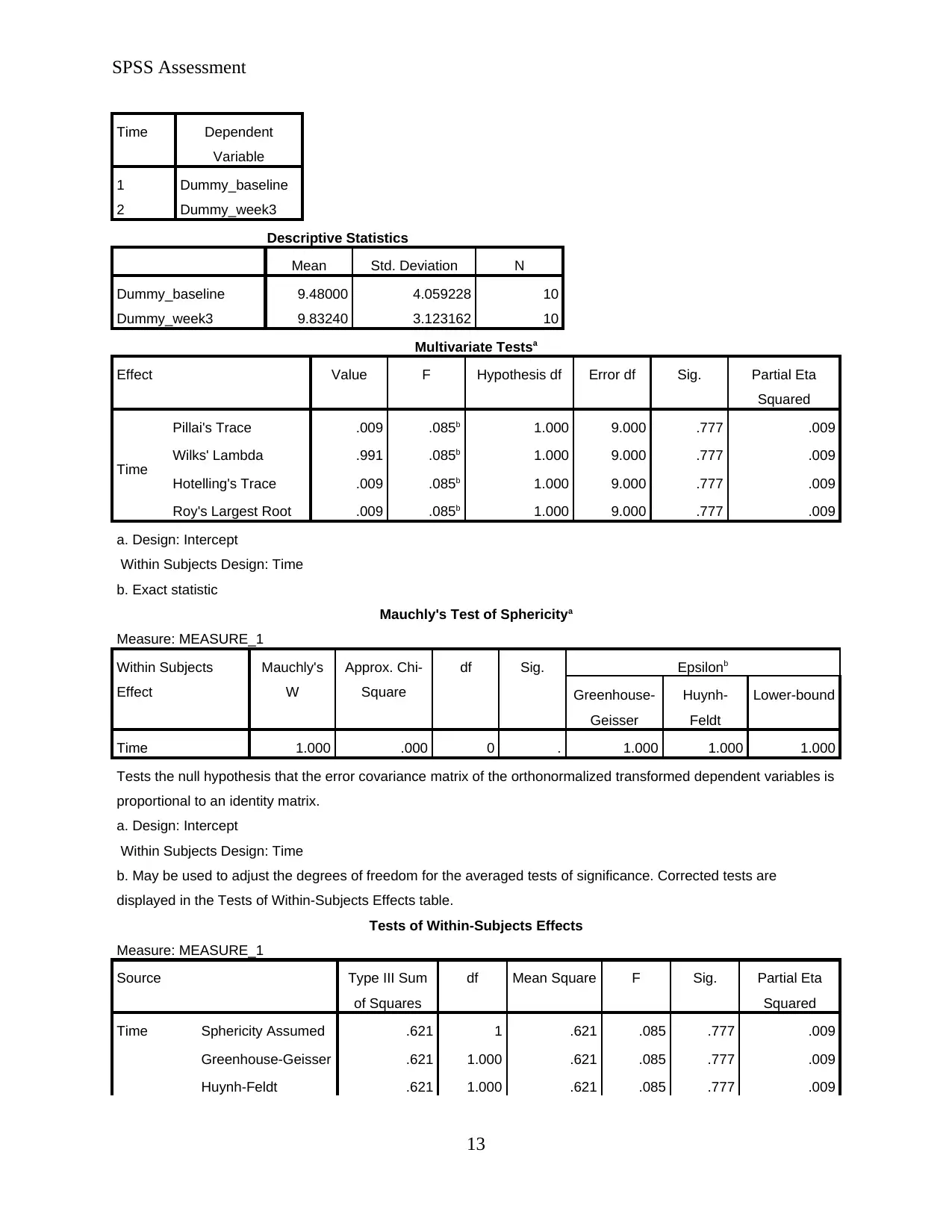
Descriptive statistics for two dummy variables are computed which are representing the
statistics of baseline and week 3 but of only those participants which were not given any
additional theory along with Ketamine treatment. The mean of baseline is 9.48 and mean of
week 3 is 9.83. By looking at these two mean values, it is clear that both of these variables has
different means of depression severity but to identify whether this difference is significant or not,
the table of “Tests of Within – Subjects Effects” will be considered.
4

SPSS Assessment
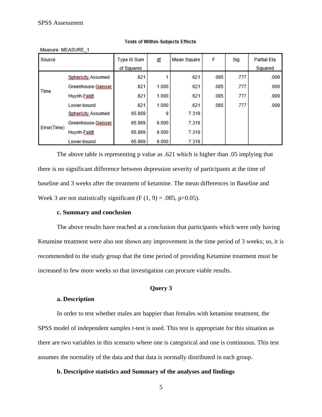
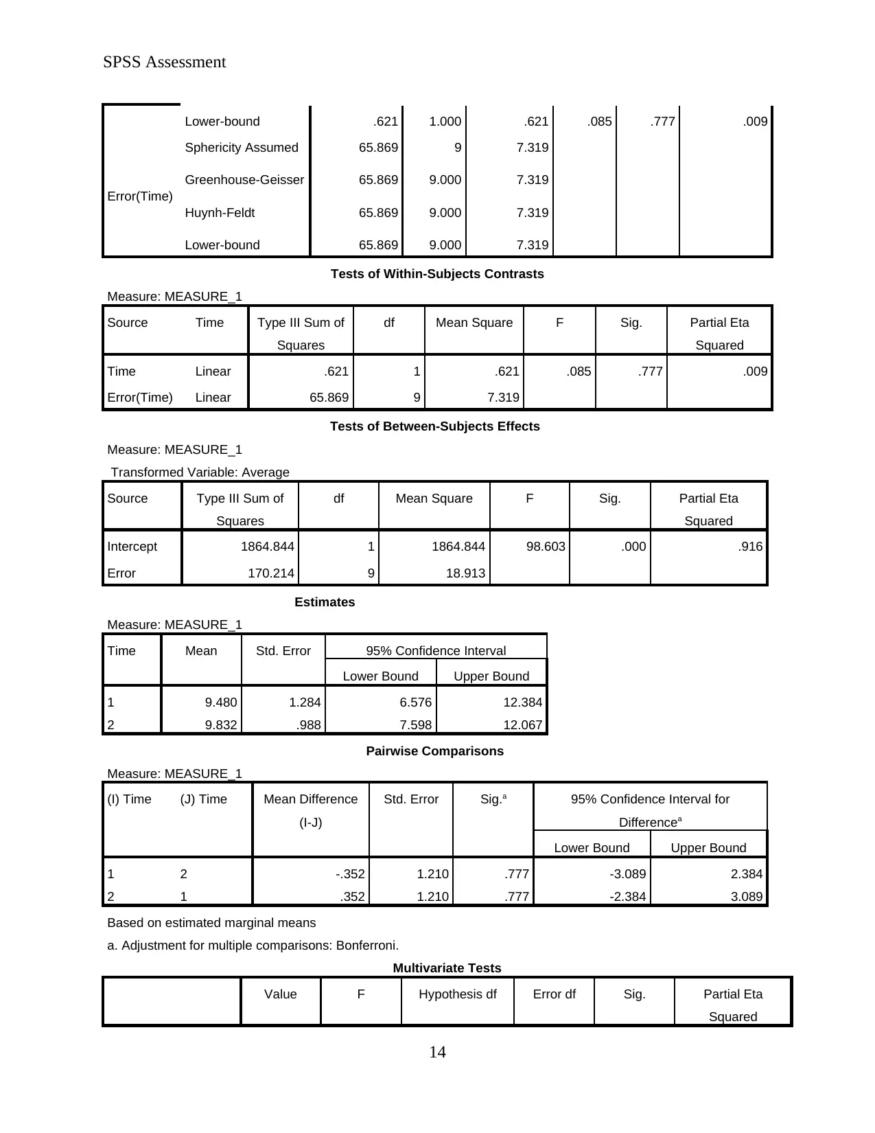
The above table is representing p value as .621 which is higher than .05 implying that
there is no significant difference between depression severity of participants at the time of
baseline and 3 weeks after the treatment of ketamine. The mean differences in Baseline and
Week 3 are not statistically significant (F (1, 9) = .085, p>0.05).
c. Summary and conclusion
The above results have reached at a conclusion that participants which were only having
Ketamine treatment were also not shown any improvement in the time period of 3 weeks; so, it is
recommended to the study group that the time period of providing Ketamine treatment must be
increased to few more weeks so that investigation can procure viable results.
Query 3
a. Description
In order to test whether males are happier than females with ketamine treatment, the
SPSS model of independent samples t-test is used. This test is appropriate for this situation as
there are two variables in this scenario where one is categorical and one is continuous. This test
assumes the normality of the data and that data is normally distributed in each group.
b. Descriptive statistics and Summary of the analyses and findings
5

SPSS Assessment
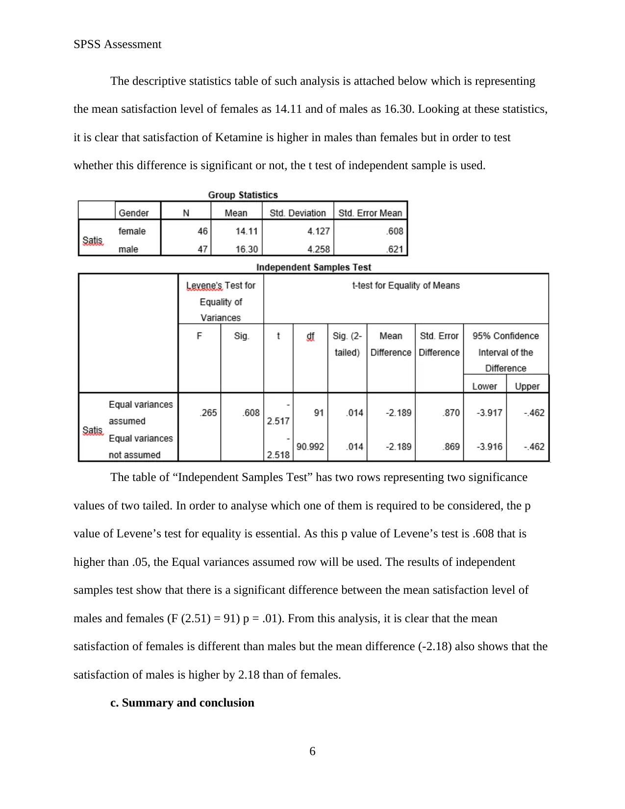
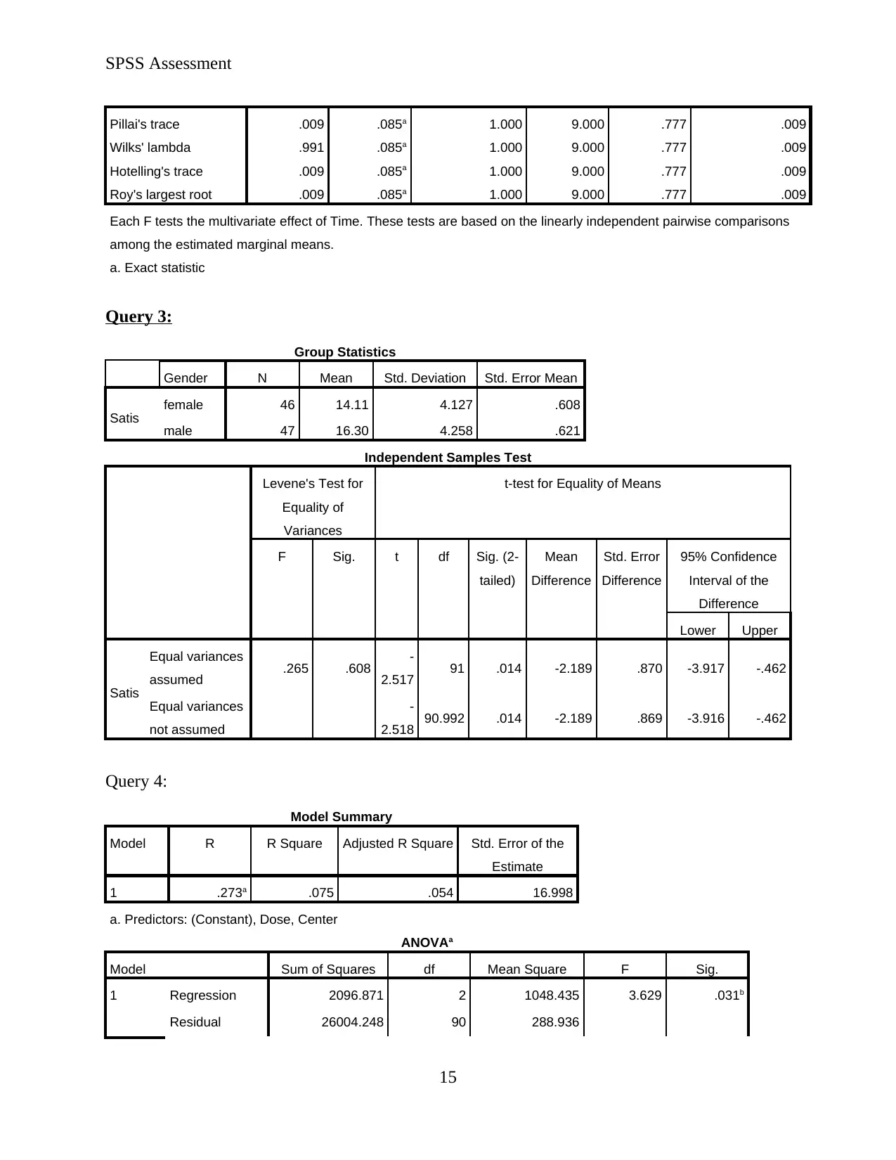
The descriptive statistics table of such analysis is attached below which is representing
the mean satisfaction level of females as 14.11 and of males as 16.30. Looking at these statistics,
it is clear that satisfaction of Ketamine is higher in males than females but in order to test
whether this difference is significant or not, the t test of independent sample is used.
The table of “Independent Samples Test” has two rows representing two significance
values of two tailed. In order to analyse which one of them is required to be considered, the p
value of Levene’s test for equality is essential. As this p value of Levene’s test is .608 that is
higher than .05, the Equal variances assumed row will be used. The results of independent
samples test show that there is a significant difference between the mean satisfaction level of
males and females (F (2.51) = 91) p = .01). From this analysis, it is clear that the mean
satisfaction of females is different than males but the mean difference (-2.18) also shows that the
satisfaction of males is higher by 2.18 than of females.
c. Summary and conclusion
6

SPSS Assessment
The output results have helped in reaching the conclusion that males are happier and
highly satisfied with the ketamine treatment so it is recommended to the research team to
conduct next study on males only.
Query 4
a. Description
In this specific query, it is required to test whether dose and centre of treatment influence
the engagement levels of participants. For this particular query, the model of regression is
selected to be used. Regression is a model which can identify the impact of various independent
variables on one dependent variable. As the query has one continuous dependent variable of
“engagement level” and two categorical independent variables, the model regression is most
appropriate. Few assumptions made under this model also justifies the selected of regression.
Regression model assumes that the relationship between variables is linear and the variance
residual is similar for all values of X. This model also assumes that every observation is
independent.
b. Descriptive statistics and Summary of the analyses and findings
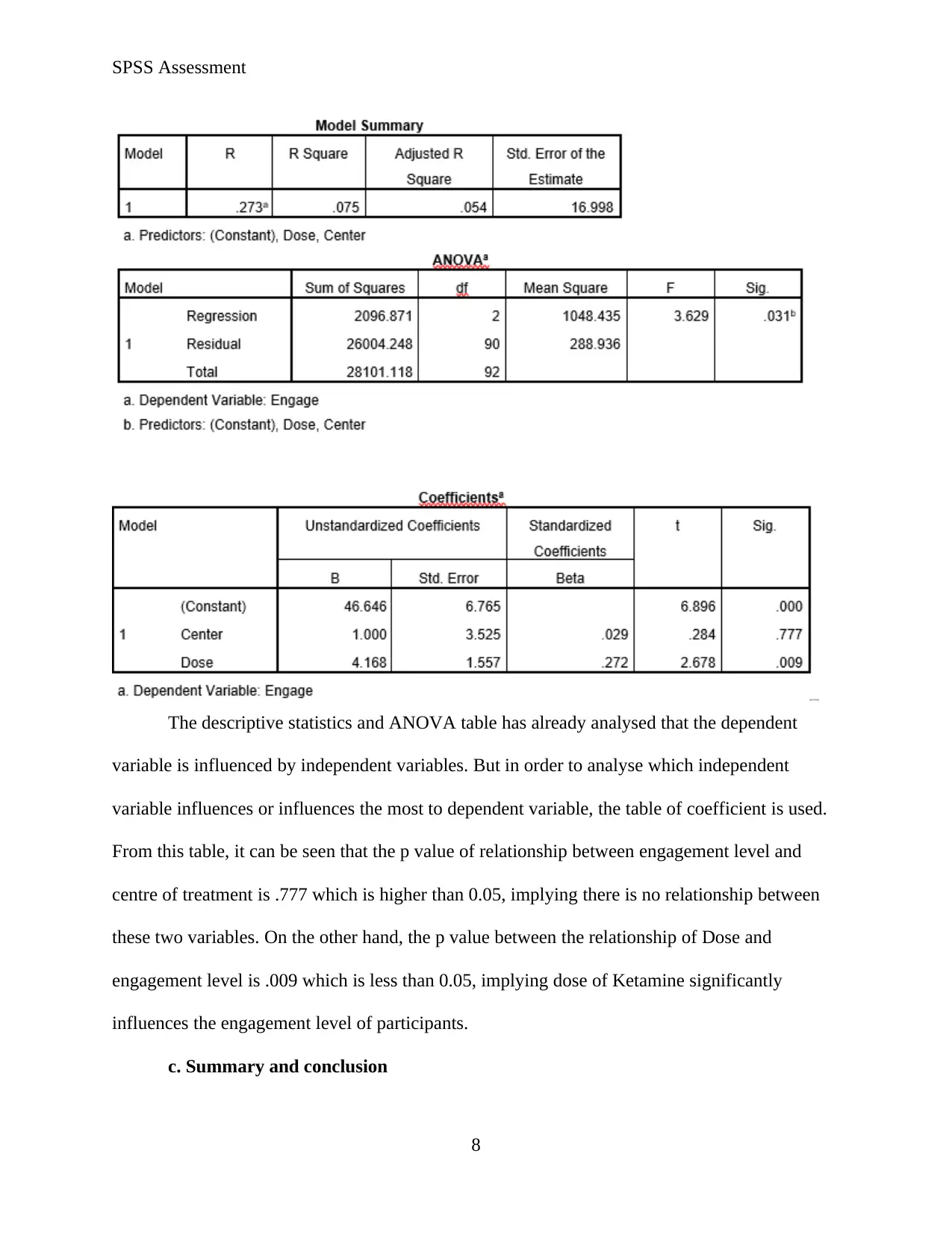
The descriptive of regression model are the R and R square values. The R value of such
analysis is .27 which represents the overall correlation between independent and dependent
variables and as the R value is .27 it represents low and weak relationship between these
variables. The value of R square represents the total variation in dependent variable due to
independent variables. The R square variable indicates that level of engagement variates only
07% by centre of treatment and dosage. Apart from these summary statistics, the ANOVA table
represents overall influence between variables. The regression model represents that there is a
significant influence of dose and centre on engagement level (F (2) = 3.62, p = 0.31). This
conclusion was achieved by looking at the p value which is lower than 0.05.
7

SPSS Assessment
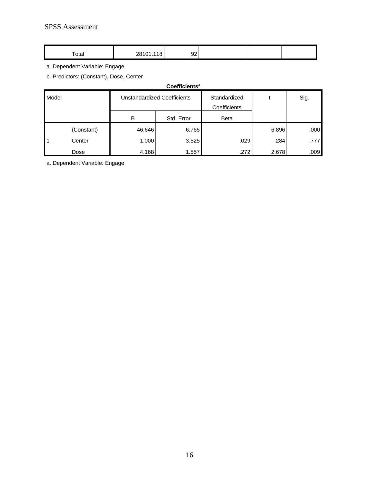
The descriptive statistics and ANOVA table has already analysed that the dependent
variable is influenced by independent variables. But in order to analyse which independent
variable influences or influences the most to dependent variable, the table of coefficient is used.
From this table, it can be seen that the p value of relationship between engagement level and
centre of treatment is .777 which is higher than 0.05, implying there is no relationship between
these two variables. On the other hand, the p value between the relationship of Dose and
engagement level is .009 which is less than 0.05, implying dose of Ketamine significantly
influences the engagement level of participants.
c. Summary and conclusion
8

SPSS Assessment
The regression model has helped to gain the conclusion that centre of study does not
influence the engagement level but the dose significantly influences engagement level.
Considering this, it is recommended that the participants which as higher engagement must give
heavier dosage to identify the level of depression severity.
9

SPSS Assessment
APPENDIX
Query 1:
Within-Subjects Factors
Measure: MEASURE_1
Time Dependent
Variable
1 baseline
2 week1
3 week2
4 week3
Descriptive Statistics
Mean Std. Deviation N
baseline 28.44086 15.749853 93
week1 38.44561 102.070488 93
week2 38.57499 102.082429 93
week3 40.44535 101.926902 93
Multivariate Testsa
Effect Value F Hypothesis df Error df Sig. Partial Eta
Squared
Time
Pillai's Trace .169 6.104b 3.000 90.000 .001 .169
Wilks' Lambda .831 6.104b 3.000 90.000 .001 .169
Hotelling's Trace .203 6.104b 3.000 90.000 .001 .169
Roy's Largest Root .203 6.104b 3.000 90.000 .001 .169
a. Design: Intercept
Within Subjects Design: Time
b. Exact statistic
Mauchly's Test of Sphericitya
Measure: MEASURE_1
Within Subjects
Effect
Mauchly's
W
Approx. Chi-
Square
df Sig. Epsilonb
Greenhouse-
Geisser
Huynh-
Feldt
Lower-bound
Time .000 918.636 5 .000 .335 .335 .333
Tests the null hypothesis that the error covariance matrix of the orthonormalized transformed dependent variables is
proportional to an identity matrix.
a. Design: Intercept
Within Subjects Design: Time
10

SPSS Assessment
b. May be used to adjust the degrees of freedom for the averaged tests of significance. Corrected tests are
displayed in the Tests of Within-Subjects Effects table.
Tests of Within-Subjects Effects
Measure: MEASURE_1
Source Type III Sum
of Squares
df Mean Square F Sig. Partial Eta
Squared
Time
Sphericity Assumed 8240.207 3 2746.736 1.055 .368 .011
Greenhouse-Geisser 8240.207 1.005 8197.039 1.055 .307 .011
Huynh-Feldt 8240.207 1.005 8195.621 1.055 .307 .011
Lower-bound 8240.207 1.000 8240.207 1.055 .307 .011
Error(Time)
Sphericity Assumed 718257.193 276 2602.381
Greenhouse-Geisser 718257.193 92.485 7766.244
Huynh-Feldt 718257.193 92.501 7764.900
Lower-bound 718257.193 92.000 7807.143
Tests of Within-Subjects Contrasts
Measure: MEASURE_1
Source Time Type III Sum of
Squares
df Mean Square F Sig. Partial Eta
Squared
Time
Linear 6074.325 1 6074.325 1.302 .257 .014
Quadratic 1538.412 1 1538.412 .588 .445 .006
Cubic 627.471 1 627.471 1.195 .277 .013
Error(Time)
Linear 429200.054 92 4665.218
Quadratic 240730.056 92 2616.631
Cubic 48327.083 92 525.294
Tests of Between-Subjects Effects
Measure: MEASURE_1
Transformed Variable: Average
Source Type III Sum of
Squares
df Mean Square F Sig. Partial Eta
Squared
Intercept 494964.584 1 494964.584 20.912 .000 .185
Error 2177567.746 92 23669.215
Estimates
Measure: MEASURE_1
Time Mean Std. Error 95% Confidence Interval
Lower Bound Upper Bound
11

SPSS Assessment
1 28.441 1.633 25.197 31.685
2 38.446 10.584 17.424 59.467
3 38.575 10.585 17.551 59.599
4 40.445 10.569 19.454 61.437
Pairwise Comparisons
Measure: MEASURE_1
(I) Time (J) Time Mean Difference
(I-J)
Std. Error Sig.b 95% Confidence Interval for
Differenceb
Lower Bound Upper Bound
1
2 -10.005 10.575 1.000 -38.521 18.512
3 -10.134 10.574 1.000 -38.647 18.379
4 -12.004 10.558 1.000 -40.476 16.467
2
1 10.005 10.575 1.000 -18.512 38.521
3 -.129 .377 1.000 -1.146 .887
4 -2.000* .490 .001 -3.321 -.678
3
1 10.134 10.574 1.000 -18.379 38.647
2 .129 .377 1.000 -.887 1.146
4 -1.870* .529 .004 -3.296 -.445
4
1 12.004 10.558 1.000 -16.467 40.476
2 2.000* .490 .001 .678 3.321
3 1.870* .529 .004 .445 3.296
Based on estimated marginal means
*. The mean difference is significant at the .05 level.
b. Adjustment for multiple comparisons: Bonferroni.
Multivariate Tests
Value F Hypothesis df Error df Sig. Partial Eta
Squared
Pillai's trace .169 6.104a 3.000 90.000 .001 .169
Wilks' lambda .831 6.104a 3.000 90.000 .001 .169
Hotelling's trace .203 6.104a 3.000 90.000 .001 .169
Roy's largest root .203 6.104a 3.000 90.000 .001 .169
Each F tests the multivariate effect of Time. These tests are based on the linearly independent pairwise comparisons
among the estimated marginal means.
a. Exact statistic
Query 2:
Within-Subjects Factors
Measure: MEASURE_1
12

SPSS Assessment
Time Dependent
Variable
1 Dummy_baseline
2 Dummy_week3
Descriptive Statistics
Mean Std. Deviation N
Dummy_baseline 9.48000 4.059228 10
Dummy_week3 9.83240 3.123162 10
Multivariate Testsa
Effect Value F Hypothesis df Error df Sig. Partial Eta
Squared
Time
Pillai's Trace .009 .085b 1.000 9.000 .777 .009
Wilks' Lambda .991 .085b 1.000 9.000 .777 .009
Hotelling's Trace .009 .085b 1.000 9.000 .777 .009
Roy's Largest Root .009 .085b 1.000 9.000 .777 .009
a. Design: Intercept
Within Subjects Design: Time
b. Exact statistic
Mauchly's Test of Sphericitya
Measure: MEASURE_1
Within Subjects
Effect
Mauchly's
W
Approx. Chi-
Square
df Sig. Epsilonb
Greenhouse-
Geisser
Huynh-
Feldt
Lower-bound
Time 1.000 .000 0 . 1.000 1.000 1.000
Tests the null hypothesis that the error covariance matrix of the orthonormalized transformed dependent variables is
proportional to an identity matrix.
a. Design: Intercept
Within Subjects Design: Time
b. May be used to adjust the degrees of freedom for the averaged tests of significance. Corrected tests are
displayed in the Tests of Within-Subjects Effects table.
Tests of Within-Subjects Effects
Measure: MEASURE_1
Source Type III Sum
of Squares
df Mean Square F Sig. Partial Eta
Squared
Time Sphericity Assumed .621 1 .621 .085 .777 .009
Greenhouse-Geisser .621 1.000 .621 .085 .777 .009
Huynh-Feldt .621 1.000 .621 .085 .777 .009
13

SPSS Assessment
Lower-bound .621 1.000 .621 .085 .777 .009
Error(Time)
Sphericity Assumed 65.869 9 7.319
Greenhouse-Geisser 65.869 9.000 7.319
Huynh-Feldt 65.869 9.000 7.319
Lower-bound 65.869 9.000 7.319
Tests of Within-Subjects Contrasts
Measure: MEASURE_1
Source Time Type III Sum of
Squares
df Mean Square F Sig. Partial Eta
Squared
Time Linear .621 1 .621 .085 .777 .009
Error(Time) Linear 65.869 9 7.319
Tests of Between-Subjects Effects
Measure: MEASURE_1
Transformed Variable: Average
Source Type III Sum of
Squares
df Mean Square F Sig. Partial Eta
Squared
Intercept 1864.844 1 1864.844 98.603 .000 .916
Error 170.214 9 18.913
Estimates
Measure: MEASURE_1
Time Mean Std. Error 95% Confidence Interval
Lower Bound Upper Bound
1 9.480 1.284 6.576 12.384
2 9.832 .988 7.598 12.067
Pairwise Comparisons
Measure: MEASURE_1
(I) Time (J) Time Mean Difference
(I-J)
Std. Error Sig.a 95% Confidence Interval for
Differencea
Lower Bound Upper Bound
1 2 -.352 1.210 .777 -3.089 2.384
2 1 .352 1.210 .777 -2.384 3.089
Based on estimated marginal means
a. Adjustment for multiple comparisons: Bonferroni.
Multivariate Tests
Value F Hypothesis df Error df Sig. Partial Eta
Squared
14

SPSS Assessment
Pillai's trace .009 .085a 1.000 9.000 .777 .009
Wilks' lambda .991 .085a 1.000 9.000 .777 .009
Hotelling's trace .009 .085a 1.000 9.000 .777 .009
Roy's largest root .009 .085a 1.000 9.000 .777 .009
Each F tests the multivariate effect of Time. These tests are based on the linearly independent pairwise comparisons
among the estimated marginal means.
a. Exact statistic
Query 3:
Group Statistics
Gender N Mean Std. Deviation Std. Error Mean
Satis female 46 14.11 4.127 .608
male 47 16.30 4.258 .621
Independent Samples Test
Levene's Test for
Equality of
Variances
t-test for Equality of Means
F Sig. t df Sig. (2-
tailed)
Mean
Difference
Std. Error
Difference
95% Confidence
Interval of the
Difference
Lower Upper
Satis
Equal variances
assumed .265 .608 -
2.517 91 .014 -2.189 .870 -3.917 -.462
Equal variances
not assumed
-
2.518 90.992 .014 -2.189 .869 -3.916 -.462
Query 4:
Model Summary
Model R R Square Adjusted R Square Std. Error of the
Estimate
1 .273a .075 .054 16.998
a. Predictors: (Constant), Dose, Center
ANOVAa
Model Sum of Squares df Mean Square F Sig.
1 Regression 2096.871 2 1048.435 3.629 .031b
Residual 26004.248 90 288.936
15

SPSS Assessment
Total 28101.118 92
a. Dependent Variable: Engage
b. Predictors: (Constant), Dose, Center
Coefficientsa
Model Unstandardized Coefficients Standardized
Coefficients
t Sig.
B Std. Error Beta
1
(Constant) 46.646 6.765 6.896 .000
Center 1.000 3.525 .029 .284 .777
Dose 4.168 1.557 .272 2.678 .009
a. Dependent Variable: Engage
16