(Solved) SPSS Assignment Sample

SPSS

TABLE OF CONTENTS
5.10..............................................................................................................................................4
a....................................................................................................................................................4
5.30..............................................................................................................................................4
5.36..............................................................................................................................................5
a....................................................................................................................................................5
b...................................................................................................................................................5
c....................................................................................................................................................5
d...................................................................................................................................................5
9.24..............................................................................................................................................6
a....................................................................................................................................................6
b...................................................................................................................................................9
c..................................................................................................................................................10
d.................................................................................................................................................11
9.28............................................................................................................................................12
11.8............................................................................................................................................13
a..................................................................................................................................................13
b.................................................................................................................................................13
c..................................................................................................................................................13
d.................................................................................................................................................14
11.12..........................................................................................................................................14
a..................................................................................................................................................14
b.................................................................................................................................................14
11.14..........................................................................................................................................14

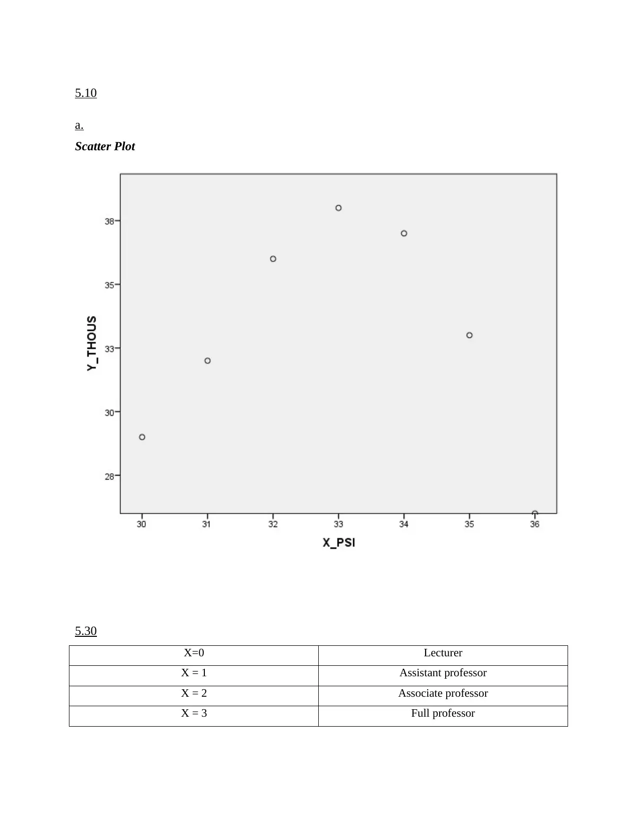
5.10
a.
Scatter Plot
5.30
X=0 Lecturer
X = 1 Assistant professor
X = 2 Associate professor
X = 3 Full professor

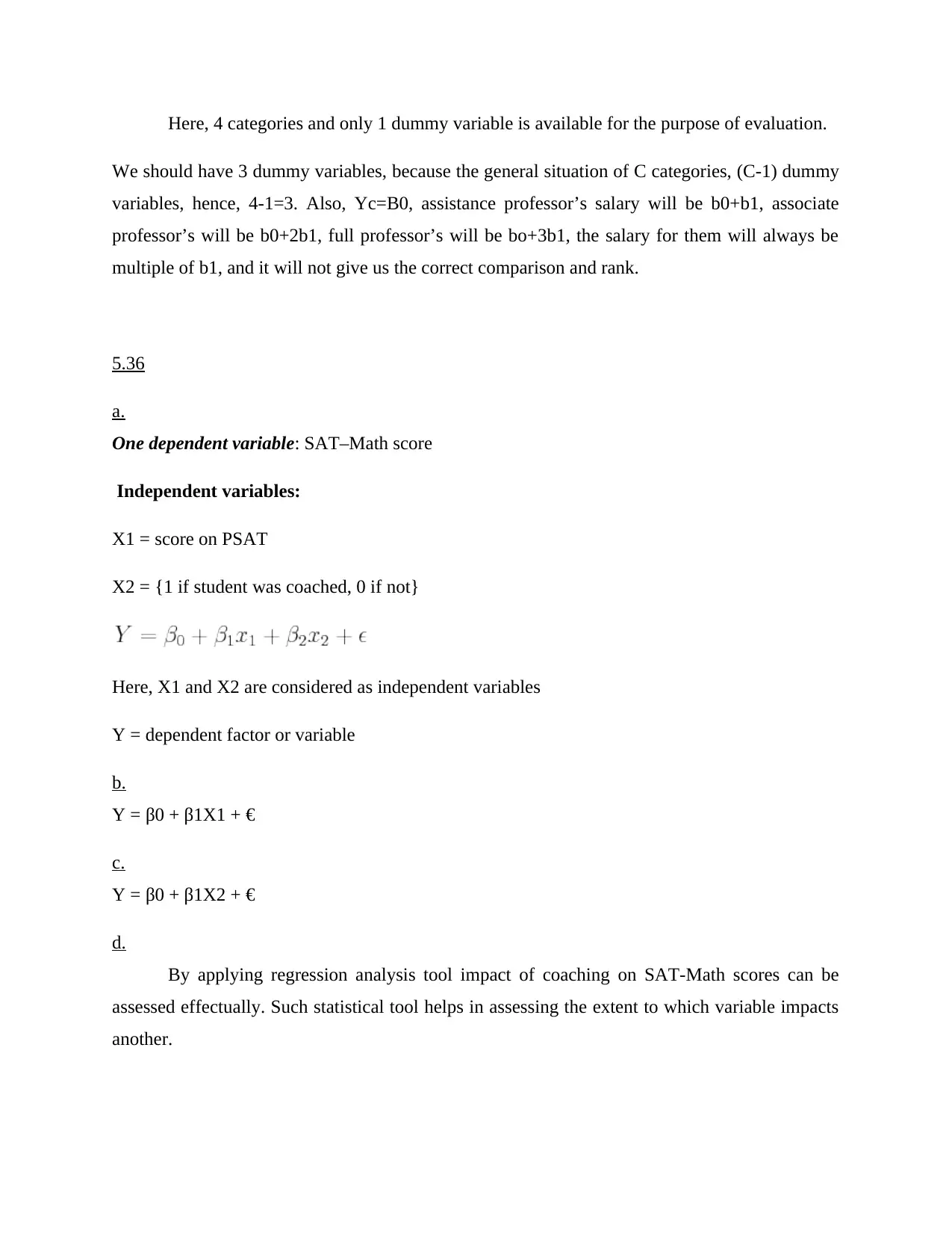
Here, 4 categories and only 1 dummy variable is available for the purpose of evaluation.
We should have 3 dummy variables, because the general situation of C categories, (C-1) dummy
variables, hence, 4-1=3. Also, Yc=B0, assistance professor’s salary will be b0+b1, associate
professor’s will be b0+2b1, full professor’s will be bo+3b1, the salary for them will always be
multiple of b1, and it will not give us the correct comparison and rank.
5.36
a.
One dependent variable: SAT–Math score
Independent variables:
X1 = score on PSAT
X2 = {1 if student was coached, 0 if not}
Here, X1 and X2 are considered as independent variables
Y = dependent factor or variable
b.
Y = β0 + β1X1 + €
c.
Y = β0 + β1X2 + €
d.
By applying regression analysis tool impact of coaching on SAT-Math scores can be
assessed effectually. Such statistical tool helps in assessing the extent to which variable impacts
another.

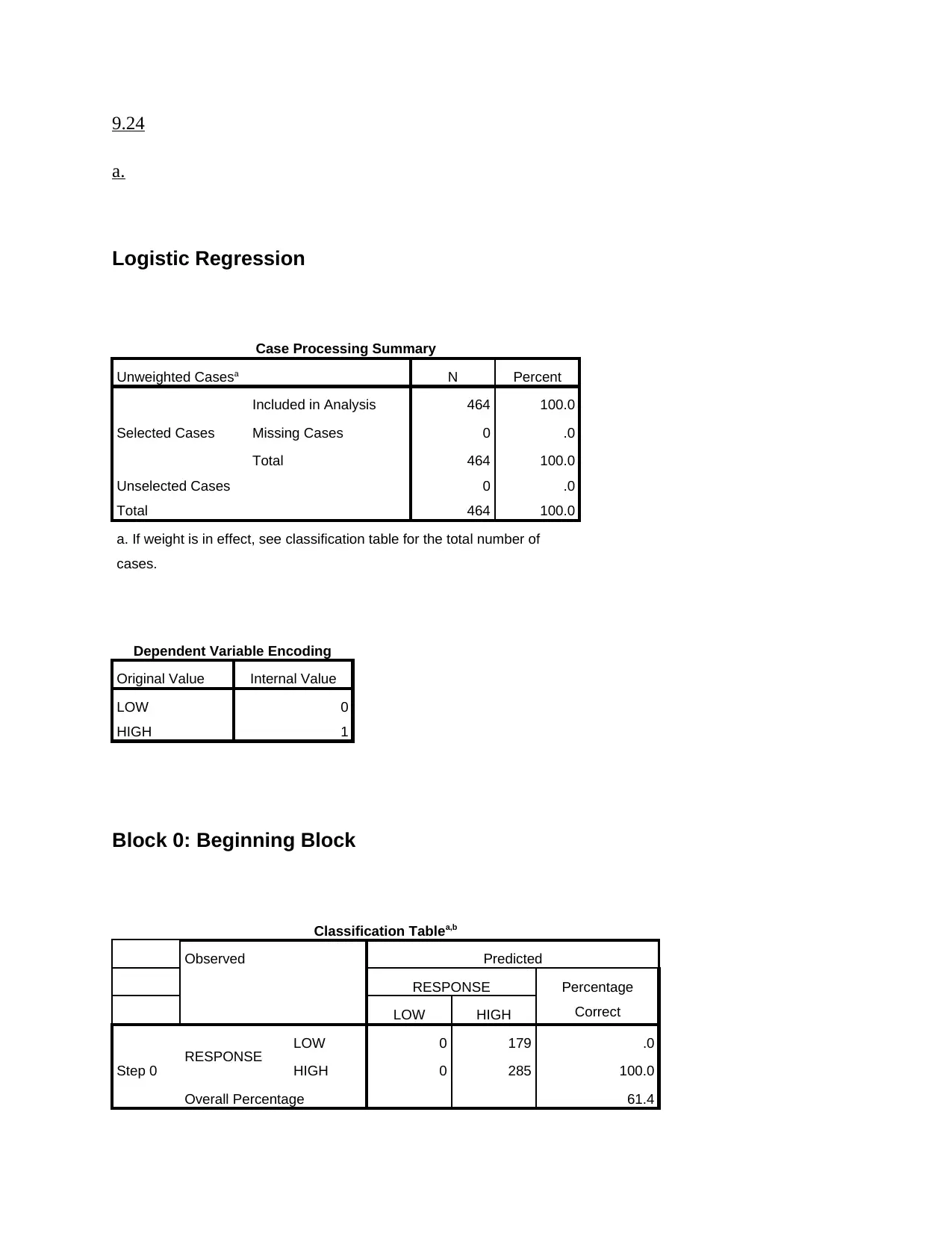
9.24
a.
Logistic Regression
Case Processing Summary
Unweighted Casesa N Percent
Selected Cases
Included in Analysis 464 100.0
Missing Cases 0 .0
Total 464 100.0
Unselected Cases 0 .0
Total 464 100.0
a. If weight is in effect, see classification table for the total number of
cases.
Dependent Variable Encoding
Original Value Internal Value
LOW 0
HIGH 1
Block 0: Beginning Block
Classification Tablea,b
Observed Predicted
RESPONSE Percentage
CorrectLOW HIGH
Step 0 RESPONSE LOW 0 179 .0
HIGH 0 285 100.0
Overall Percentage 61.4

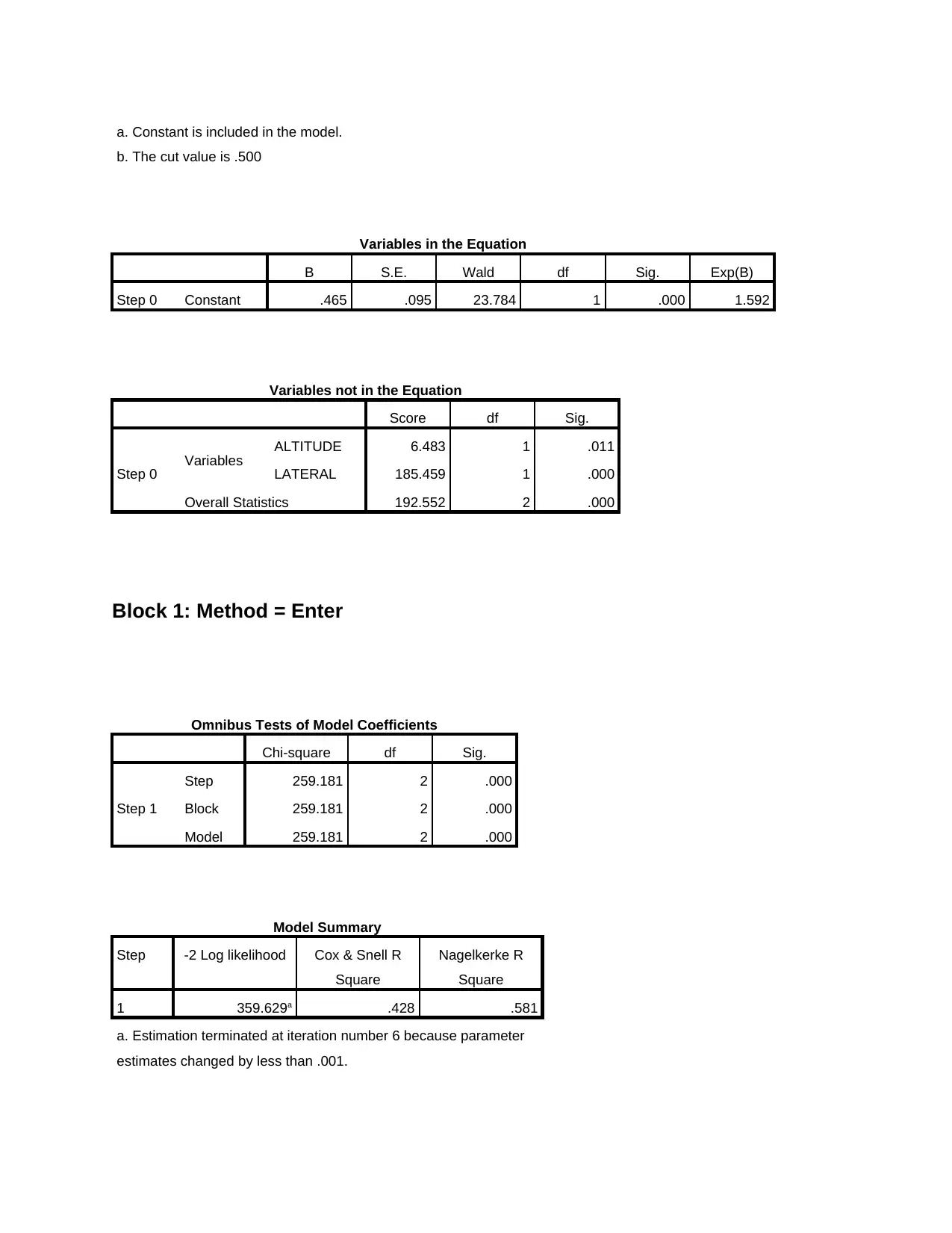
a. Constant is included in the model.
b. The cut value is .500
Variables in the Equation
B S.E. Wald df Sig. Exp(B)
Step 0 Constant .465 .095 23.784 1 .000 1.592
Variables not in the Equation
Score df Sig.
Step 0 Variables ALTITUDE 6.483 1 .011
LATERAL 185.459 1 .000
Overall Statistics 192.552 2 .000
Block 1: Method = Enter
Omnibus Tests of Model Coefficients
Chi-square df Sig.
Step 1
Step 259.181 2 .000
Block 259.181 2 .000
Model 259.181 2 .000
Model Summary
Step -2 Log likelihood Cox & Snell R
Square
Nagelkerke R
Square
1 359.629a .428 .581
a. Estimation terminated at iteration number 6 because parameter
estimates changed by less than .001.

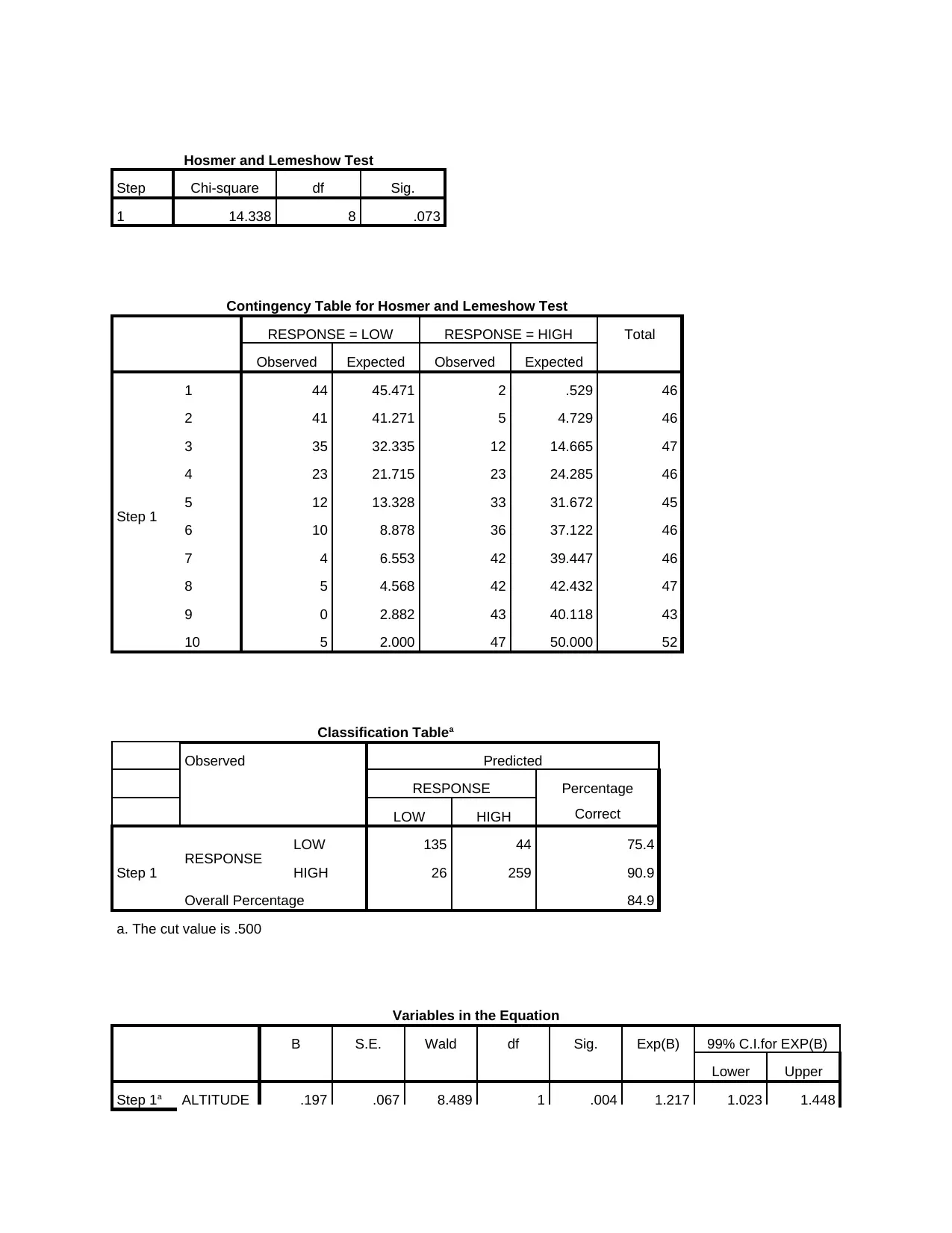
Hosmer and Lemeshow Test
Step Chi-square df Sig.
1 14.338 8 .073
Contingency Table for Hosmer and Lemeshow Test
RESPONSE = LOW RESPONSE = HIGH Total
Observed Expected Observed Expected
Step 1
1 44 45.471 2 .529 46
2 41 41.271 5 4.729 46
3 35 32.335 12 14.665 47
4 23 21.715 23 24.285 46
5 12 13.328 33 31.672 45
6 10 8.878 36 37.122 46
7 4 6.553 42 39.447 46
8 5 4.568 42 42.432 47
9 0 2.882 43 40.118 43
10 5 2.000 47 50.000 52
Classification Tablea
Observed Predicted
RESPONSE Percentage
CorrectLOW HIGH
Step 1 RESPONSE LOW 135 44 75.4
HIGH 26 259 90.9
Overall Percentage 84.9
a. The cut value is .500
Variables in the Equation
B S.E. Wald df Sig. Exp(B) 99% C.I.for EXP(B)
Lower Upper
Step 1a ALTITUDE .197 .067 8.489 1 .004 1.217 1.023 1.448

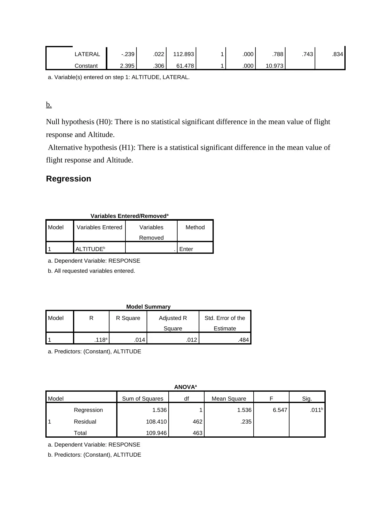
LATERAL -.239 .022 112.893 1 .000 .788 .743 .834
Constant 2.395 .306 61.478 1 .000 10.973
a. Variable(s) entered on step 1: ALTITUDE, LATERAL.
b.
Null hypothesis (H0): There is no statistical significant difference in the mean value of flight
response and Altitude.
Alternative hypothesis (H1): There is a statistical significant difference in the mean value of
flight response and Altitude.
Regression
Variables Entered/Removeda
Model Variables Entered Variables
Removed
Method
1 ALTITUDEb . Enter
a. Dependent Variable: RESPONSE
b. All requested variables entered.
Model Summary
Model R R Square Adjusted R
Square
Std. Error of the
Estimate
1 .118a .014 .012 .484
a. Predictors: (Constant), ALTITUDE
ANOVAa
Model Sum of Squares df Mean Square F Sig.
1
Regression 1.536 1 1.536 6.547 .011b
Residual 108.410 462 .235
Total 109.946 463
a. Dependent Variable: RESPONSE
b. Predictors: (Constant), ALTITUDE

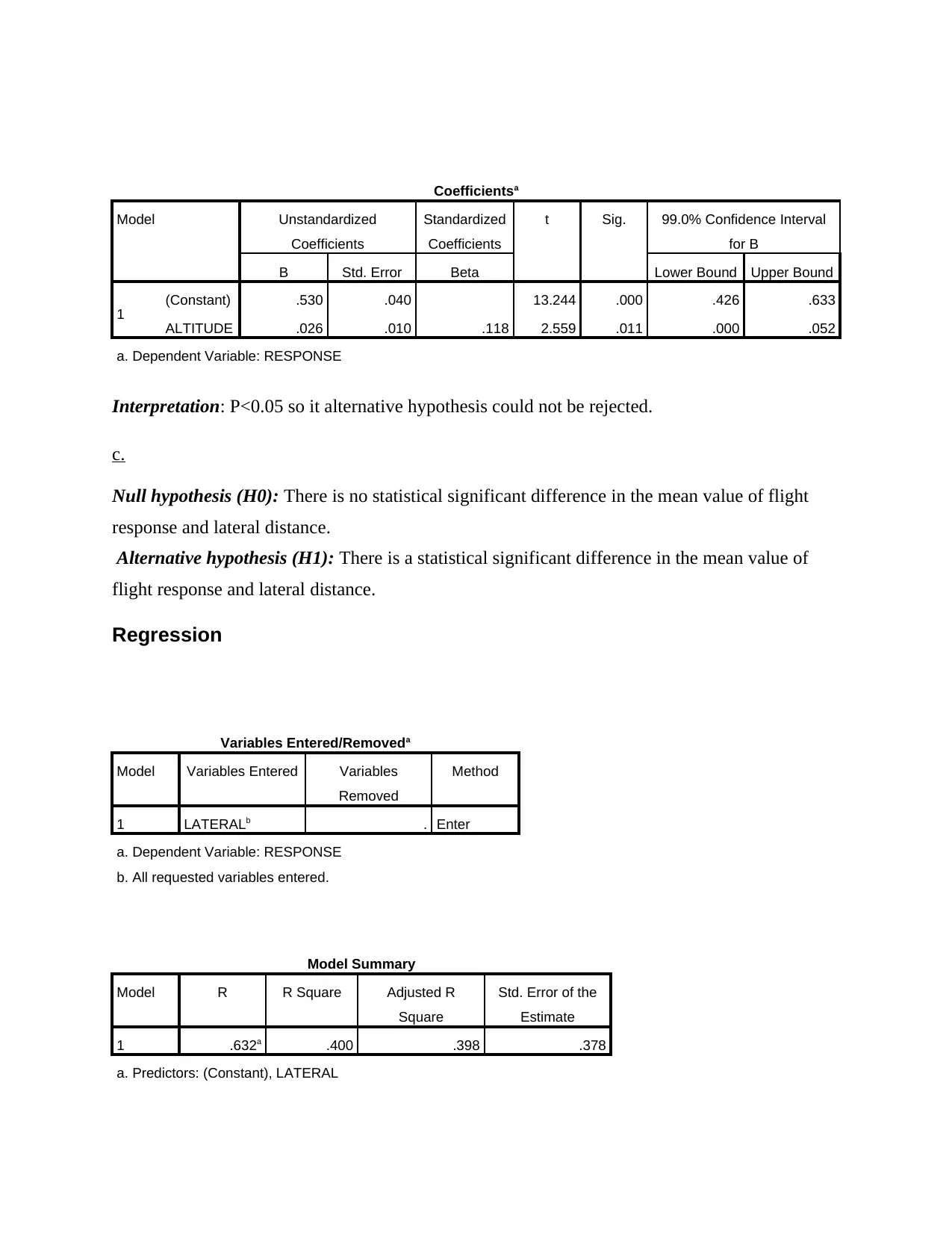
Coefficientsa
Model Unstandardized
Coefficients
Standardized
Coefficients
t Sig. 99.0% Confidence Interval
for B
B Std. Error Beta Lower Bound Upper Bound
1 (Constant) .530 .040 13.244 .000 .426 .633
ALTITUDE .026 .010 .118 2.559 .011 .000 .052
a. Dependent Variable: RESPONSE
Interpretation: P<0.05 so it alternative hypothesis could not be rejected.
c.
Null hypothesis (H0): There is no statistical significant difference in the mean value of flight
response and lateral distance.
Alternative hypothesis (H1): There is a statistical significant difference in the mean value of
flight response and lateral distance.
Regression
Variables Entered/Removeda
Model Variables Entered Variables
Removed
Method
1 LATERALb . Enter
a. Dependent Variable: RESPONSE
b. All requested variables entered.
Model Summary
Model R R Square Adjusted R
Square
Std. Error of the
Estimate
1 .632a .400 .398 .378
a. Predictors: (Constant), LATERAL

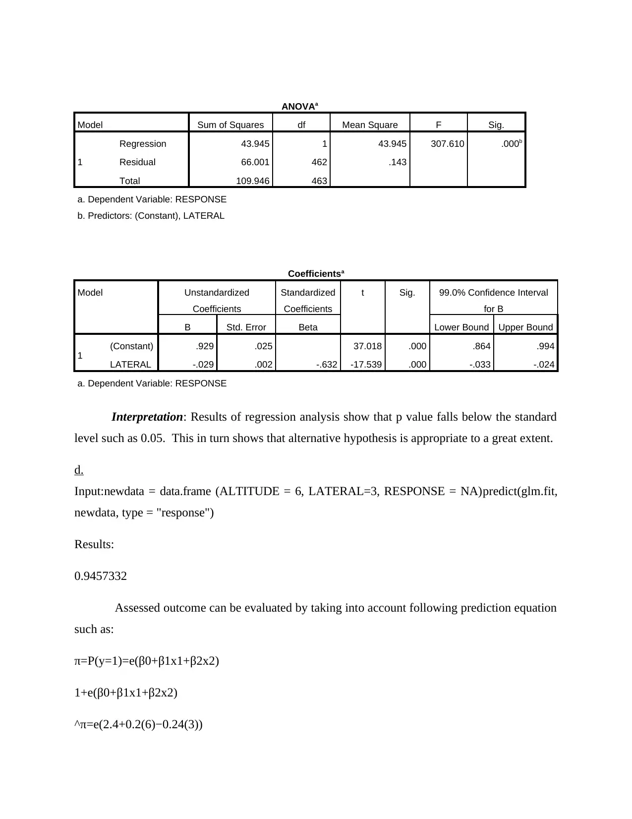
ANOVAa
Model Sum of Squares df Mean Square F Sig.
1
Regression 43.945 1 43.945 307.610 .000b
Residual 66.001 462 .143
Total 109.946 463
a. Dependent Variable: RESPONSE
b. Predictors: (Constant), LATERAL
Coefficientsa
Model Unstandardized
Coefficients
Standardized
Coefficients
t Sig. 99.0% Confidence Interval
for B
B Std. Error Beta Lower Bound Upper Bound
1 (Constant) .929 .025 37.018 .000 .864 .994
LATERAL -.029 .002 -.632 -17.539 .000 -.033 -.024
a. Dependent Variable: RESPONSE
Interpretation: Results of regression analysis show that p value falls below the standard
level such as 0.05. This in turn shows that alternative hypothesis is appropriate to a great extent.
d.
Input:newdata = data.frame (ALTITUDE = 6, LATERAL=3, RESPONSE = NA)predict(glm.fit,
newdata, type = "response")
Results:
0.9457332
Assessed outcome can be evaluated by taking into account following prediction equation
such as:
π=P(y=1)=e(β0+β1x1+β2x2)
1+e(β0+β1x1+β2x2)
^π=e(2.4+0.2(6)−0.24(3))

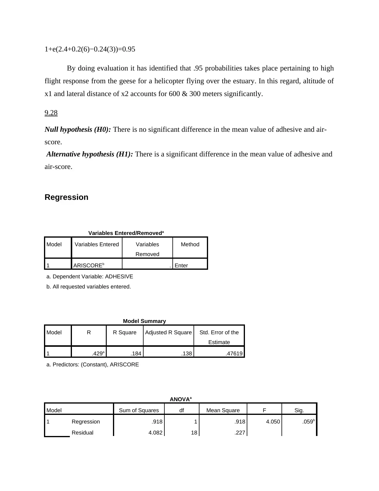
1+e(2.4+0.2(6)−0.24(3))=0.95
By doing evaluation it has identified that .95 probabilities takes place pertaining to high
flight response from the geese for a helicopter flying over the estuary. In this regard, altitude of
x1 and lateral distance of x2 accounts for 600 & 300 meters significantly.
9.28
Null hypothesis (H0): There is no significant difference in the mean value of adhesive and air-
score.
Alternative hypothesis (H1): There is a significant difference in the mean value of adhesive and
air-score.
Regression
Variables Entered/Removeda
Model Variables Entered Variables
Removed
Method
1 ARISCOREb . Enter
a. Dependent Variable: ADHESIVE
b. All requested variables entered.
Model Summary
Model R R Square Adjusted R Square Std. Error of the
Estimate
1 .429a .184 .138 .47619
a. Predictors: (Constant), ARISCORE
ANOVAa
Model Sum of Squares df Mean Square F Sig.
1 Regression .918 1 .918 4.050 .059b
Residual 4.082 18 .227

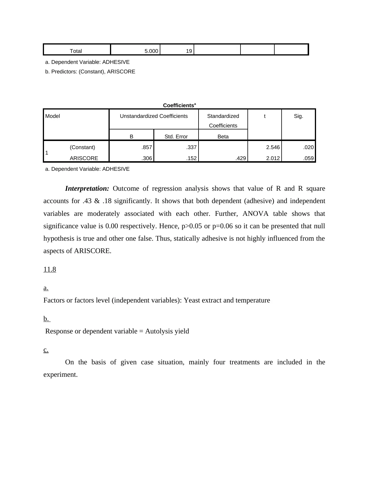
Total 5.000 19
a. Dependent Variable: ADHESIVE
b. Predictors: (Constant), ARISCORE
Coefficientsa
Model Unstandardized Coefficients Standardized
Coefficients
t Sig.
B Std. Error Beta
1 (Constant) .857 .337 2.546 .020
ARISCORE .306 .152 .429 2.012 .059
a. Dependent Variable: ADHESIVE
Interpretation: Outcome of regression analysis shows that value of R and R square
accounts for .43 & .18 significantly. It shows that both dependent (adhesive) and independent
variables are moderately associated with each other. Further, ANOVA table shows that
significance value is 0.00 respectively. Hence, p>0.05 or p=0.06 so it can be presented that null
hypothesis is true and other one false. Thus, statically adhesive is not highly influenced from the
aspects of ARISCORE.
11.8
a.
Factors or factors level (independent variables): Yeast extract and temperature
b.
Response or dependent variable = Autolysis yield
c.
On the basis of given case situation, mainly four treatments are included in the
experiment.

d.
In this, factorial design has been employed for testing the concerned hypothesis. Such
design helps in manipulating two or more independent variables simultaneously and analyzing
their impact on dependent factors.
11.12
a.
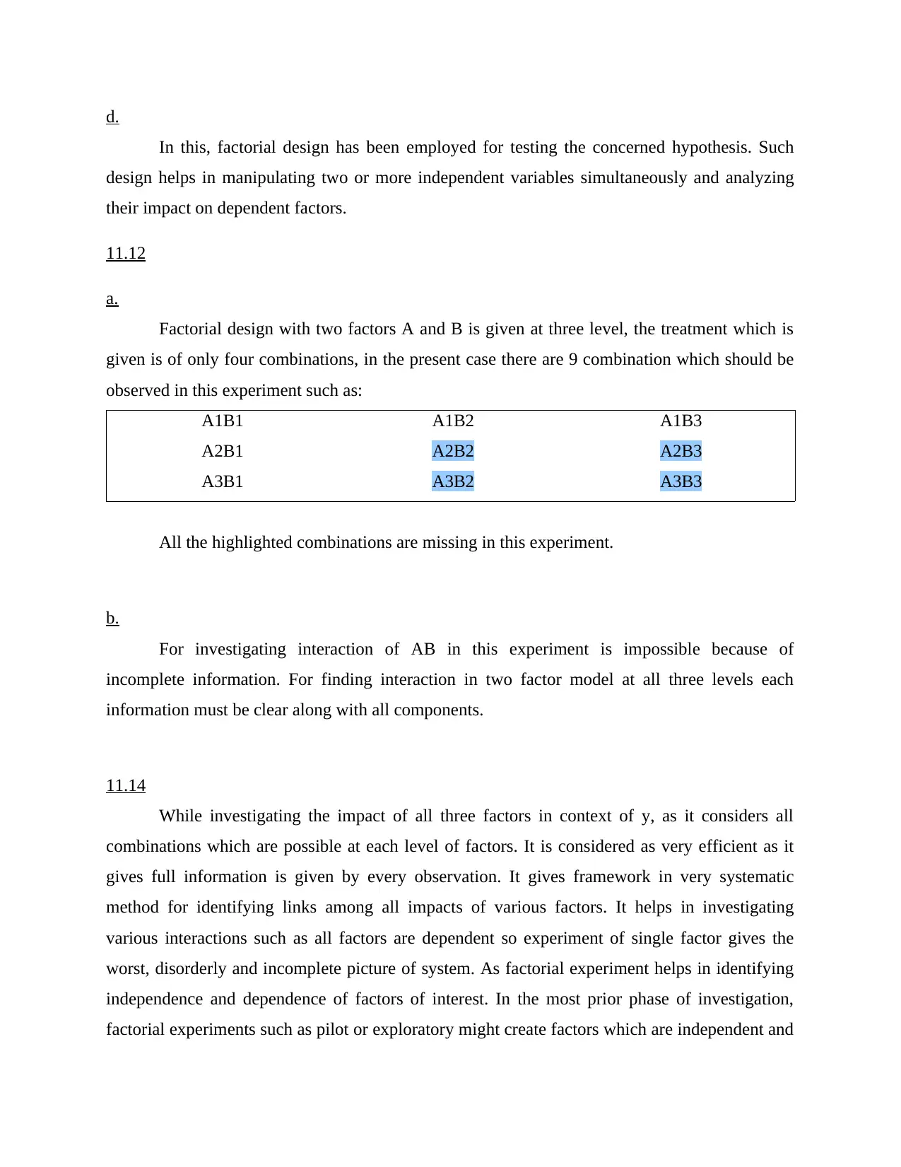
Factorial design with two factors A and B is given at three level, the treatment which is
given is of only four combinations, in the present case there are 9 combination which should be
observed in this experiment such as:
A1B1 A1B2 A1B3
A2B1 A2B2 A2B3
A3B1 A3B2 A3B3
All the highlighted combinations are missing in this experiment.
b.
For investigating interaction of AB in this experiment is impossible because of
incomplete information. For finding interaction in two factor model at all three levels each
information must be clear along with all components.
11.14
While investigating the impact of all three factors in context of y, as it considers all
combinations which are possible at each level of factors. It is considered as very efficient as it
gives full information is given by every observation. It gives framework in very systematic
method for identifying links among all impacts of various factors. It helps in investigating
various interactions such as all factors are dependent so experiment of single factor gives the
worst, disorderly and incomplete picture of system. As factorial experiment helps in identifying
independence and dependence of factors of interest. In the most prior phase of investigation,
factorial experiments such as pilot or exploratory might create factors which are independent and

they can be appropriately analysed in different experiment. In order for giving recommendations
there should be applicability of conditions of different situations of various range as different
subsidiary factors in this specific experiment can be introduced for ensuring about outcomes
which are recommended and they are applied at various range of circumstances which are
necessary.