SPSS Data Analysis
VerifiedAdded on 2022/12/28
|17
|3874
|1
AI Summary
This research analyzes the crime rates' perception and their effect on gender and age using SPSS data analysis. It explores the relationship between confidence in fairness in the criminal justice system (CJS) and trust in the police. The research findings indicate significant differences in perception between male and female participants and a strong relationship between confidence in fairness in the CJS and trust in the police among males.
Contribute Materials
Your contribution can guide someone’s learning journey. Share your
documents today.

Running head: SPSS DATA ANALYSIS
Crime rates’ perception, and their effect on Gender and age
Name:
Institution:
Crime rates’ perception, and their effect on Gender and age
Name:
Institution:
Secure Best Marks with AI Grader
Need help grading? Try our AI Grader for instant feedback on your assignments.
SPSS DATA ANALYSIS
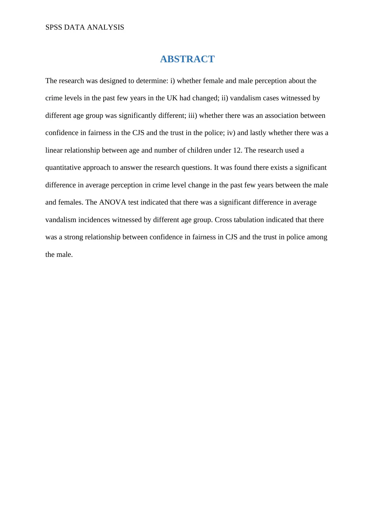
ABSTRACT
The research was designed to determine: i) whether female and male perception about the
crime levels in the past few years in the UK had changed; ii) vandalism cases witnessed by
different age group was significantly different; iii) whether there was an association between
confidence in fairness in the CJS and the trust in the police; iv) and lastly whether there was a
linear relationship between age and number of children under 12. The research used a
quantitative approach to answer the research questions. It was found there exists a significant
difference in average perception in crime level change in the past few years between the male
and females. The ANOVA test indicated that there was a significant difference in average
vandalism incidences witnessed by different age group. Cross tabulation indicated that there
was a strong relationship between confidence in fairness in CJS and the trust in police among
the male.
SPSS DATA ANALYSIS
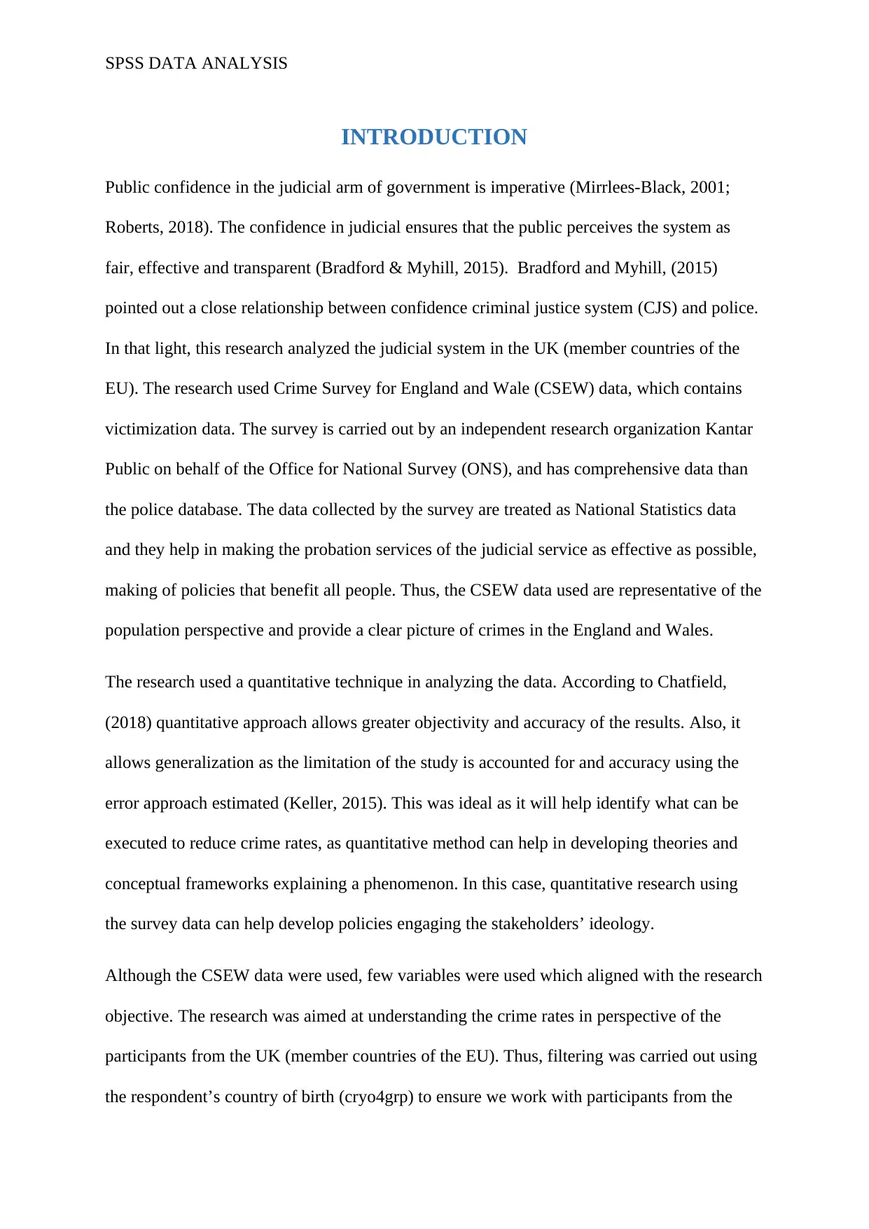
INTRODUCTION
Public confidence in the judicial arm of government is imperative (Mirrlees-Black, 2001;
Roberts, 2018). The confidence in judicial ensures that the public perceives the system as
fair, effective and transparent (Bradford & Myhill, 2015). Bradford and Myhill, (2015)
pointed out a close relationship between confidence criminal justice system (CJS) and police.
In that light, this research analyzed the judicial system in the UK (member countries of the
EU). The research used Crime Survey for England and Wale (CSEW) data, which contains
victimization data. The survey is carried out by an independent research organization Kantar
Public on behalf of the Office for National Survey (ONS), and has comprehensive data than
the police database. The data collected by the survey are treated as National Statistics data
and they help in making the probation services of the judicial service as effective as possible,
making of policies that benefit all people. Thus, the CSEW data used are representative of the
population perspective and provide a clear picture of crimes in the England and Wales.
The research used a quantitative technique in analyzing the data. According to Chatfield,
(2018) quantitative approach allows greater objectivity and accuracy of the results. Also, it
allows generalization as the limitation of the study is accounted for and accuracy using the
error approach estimated (Keller, 2015). This was ideal as it will help identify what can be
executed to reduce crime rates, as quantitative method can help in developing theories and
conceptual frameworks explaining a phenomenon. In this case, quantitative research using
the survey data can help develop policies engaging the stakeholders’ ideology.
Although the CSEW data were used, few variables were used which aligned with the research
objective. The research was aimed at understanding the crime rates in perspective of the
participants from the UK (member countries of the EU). Thus, filtering was carried out using
the respondent’s country of birth (cryo4grp) to ensure we work with participants from the
SPSS DATA ANALYSIS
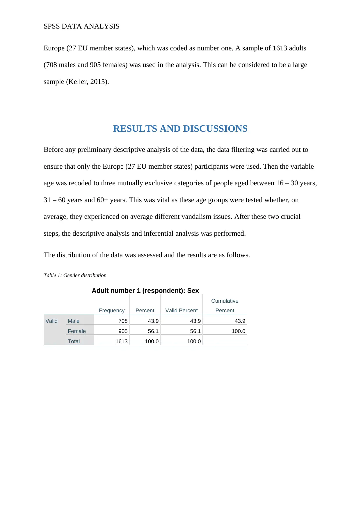
Europe (27 EU member states), which was coded as number one. A sample of 1613 adults
(708 males and 905 females) was used in the analysis. This can be considered to be a large
sample (Keller, 2015).
RESULTS AND DISCUSSIONS
Before any preliminary descriptive analysis of the data, the data filtering was carried out to
ensure that only the Europe (27 EU member states) participants were used. Then the variable
age was recoded to three mutually exclusive categories of people aged between 16 – 30 years,
31 – 60 years and 60+ years. This was vital as these age groups were tested whether, on
average, they experienced on average different vandalism issues. After these two crucial
steps, the descriptive analysis and inferential analysis was performed.
The distribution of the data was assessed and the results are as follows.
Table 1: Gender distribution
Adult number 1 (respondent): Sex
Frequency Percent Valid Percent
Cumulative
Percent
Valid Male 708 43.9 43.9 43.9
Female 905 56.1 56.1 100.0
Total 1613 100.0 100.0
Secure Best Marks with AI Grader
Need help grading? Try our AI Grader for instant feedback on your assignments.
SPSS DATA ANALYSIS
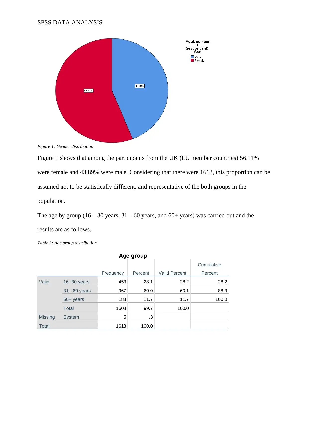
Figure 1: Gender distribution
Figure 1 shows that among the participants from the UK (EU member countries) 56.11%
were female and 43.89% were male. Considering that there were 1613, this proportion can be
assumed not to be statistically different, and representative of the both groups in the
population.
The age by group (16 – 30 years, 31 – 60 years, and 60+ years) was carried out and the
results are as follows.
Table 2: Age group distribution
Age group
Frequency Percent Valid Percent
Cumulative
Percent
Valid 16 -30 years 453 28.1 28.2 28.2
31 - 60 years 967 60.0 60.1 88.3
60+ years 188 11.7 11.7 100.0
Total 1608 99.7 100.0
Missing System 5 .3
Total 1613 100.0
SPSS DATA ANALYSIS
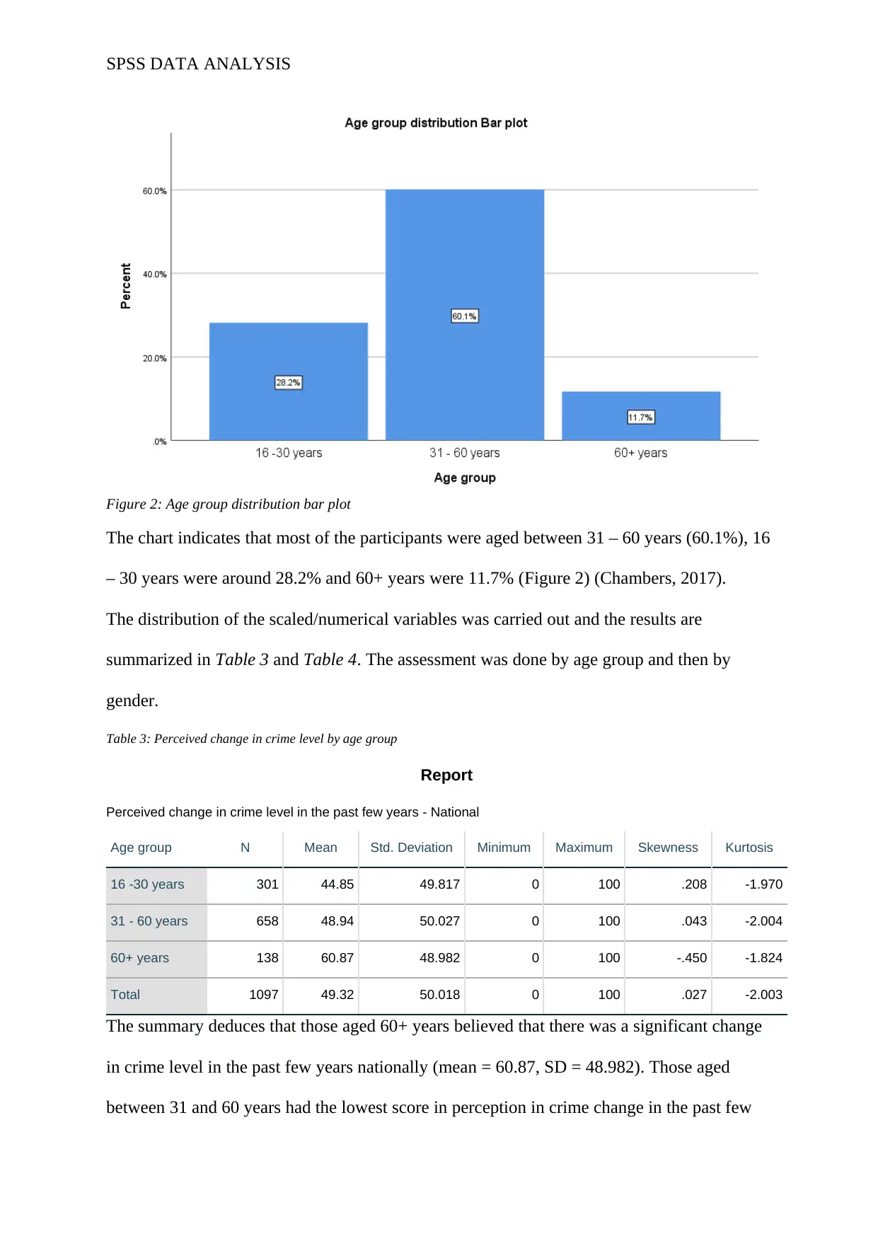
Figure 2: Age group distribution bar plot
The chart indicates that most of the participants were aged between 31 – 60 years (60.1%), 16
– 30 years were around 28.2% and 60+ years were 11.7% (Figure 2) (Chambers, 2017).
The distribution of the scaled/numerical variables was carried out and the results are
summarized in Table 3 and Table 4. The assessment was done by age group and then by
gender.
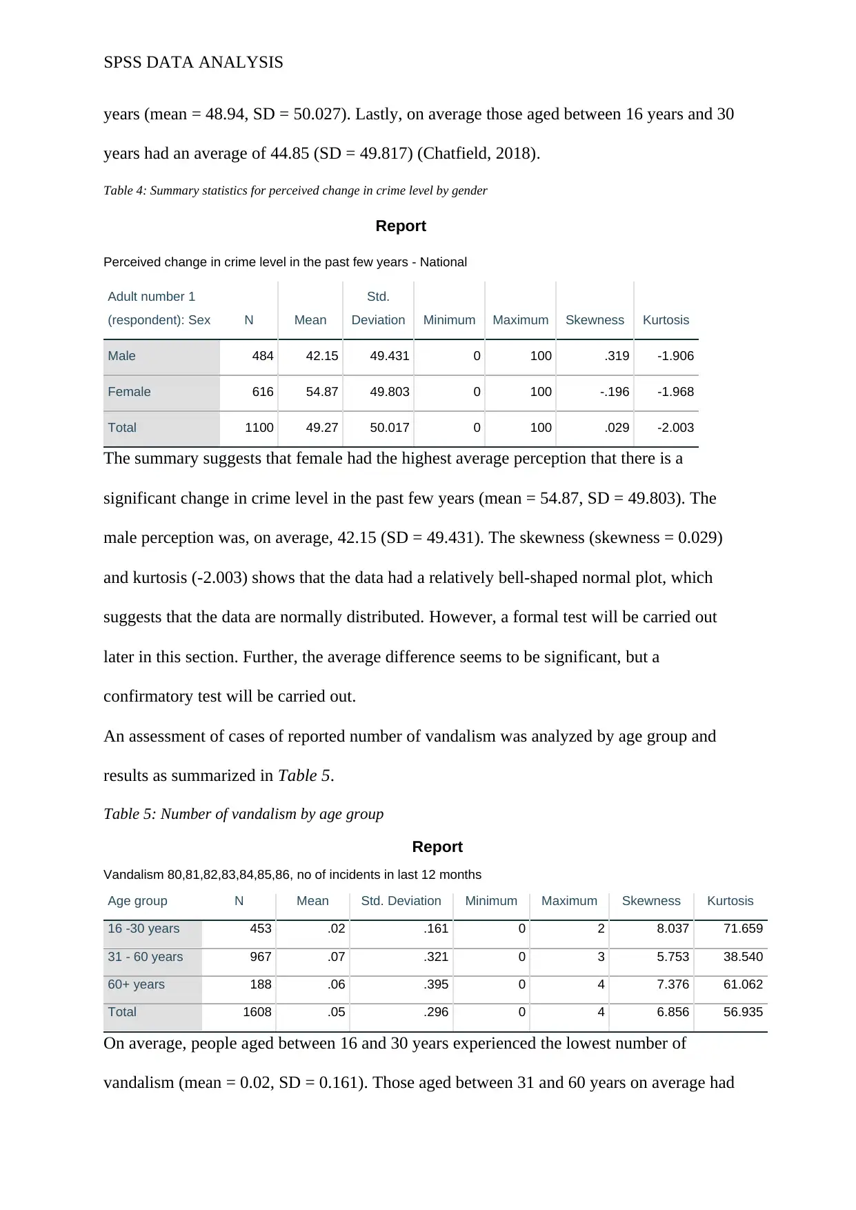
Table 3: Perceived change in crime level by age group
Report
Perceived change in crime level in the past few years - National
Age group N Mean Std. Deviation Minimum Maximum Skewness Kurtosis
16 -30 years 301 44.85 49.817 0 100 .208 -1.970
31 - 60 years 658 48.94 50.027 0 100 .043 -2.004
60+ years 138 60.87 48.982 0 100 -.450 -1.824
Total 1097 49.32 50.018 0 100 .027 -2.003
The summary deduces that those aged 60+ years believed that there was a significant change
in crime level in the past few years nationally (mean = 60.87, SD = 48.982). Those aged
between 31 and 60 years had the lowest score in perception in crime change in the past few
SPSS DATA ANALYSIS
years (mean = 48.94, SD = 50.027). Lastly, on average those aged between 16 years and 30
years had an average of 44.85 (SD = 49.817) (Chatfield, 2018).
Table 4: Summary statistics for perceived change in crime level by gender
Report
Perceived change in crime level in the past few years - National
Adult number 1
(respondent): Sex N Mean
Std.
Deviation Minimum Maximum Skewness Kurtosis
Male 484 42.15 49.431 0 100 .319 -1.906
Female 616 54.87 49.803 0 100 -.196 -1.968
Total 1100 49.27 50.017 0 100 .029 -2.003
The summary suggests that female had the highest average perception that there is a
significant change in crime level in the past few years (mean = 54.87, SD = 49.803). The
male perception was, on average, 42.15 (SD = 49.431). The skewness (skewness = 0.029)
and kurtosis (-2.003) shows that the data had a relatively bell-shaped normal plot, which
suggests that the data are normally distributed. However, a formal test will be carried out
later in this section. Further, the average difference seems to be significant, but a
confirmatory test will be carried out.
An assessment of cases of reported number of vandalism was analyzed by age group and
results as summarized in Table 5.
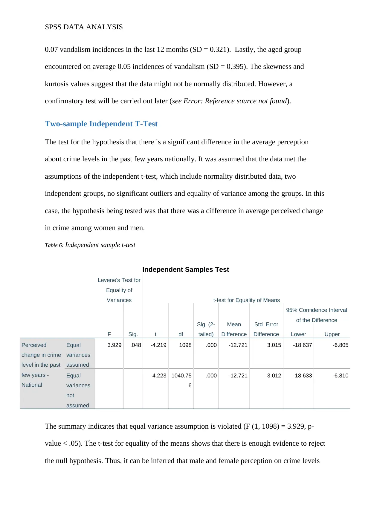
Table 5: Number of vandalism by age group
Report
Vandalism 80,81,82,83,84,85,86, no of incidents in last 12 months
Age group N Mean Std. Deviation Minimum Maximum Skewness Kurtosis
16 -30 years 453 .02 .161 0 2 8.037 71.659
31 - 60 years 967 .07 .321 0 3 5.753 38.540
60+ years 188 .06 .395 0 4 7.376 61.062
Total 1608 .05 .296 0 4 6.856 56.935
On average, people aged between 16 and 30 years experienced the lowest number of
vandalism (mean = 0.02, SD = 0.161). Those aged between 31 and 60 years on average had
Paraphrase This Document
Need a fresh take? Get an instant paraphrase of this document with our AI Paraphraser
SPSS DATA ANALYSIS
0.07 vandalism incidences in the last 12 months (SD = 0.321). Lastly, the aged group
encountered on average 0.05 incidences of vandalism (SD = 0.395). The skewness and
kurtosis values suggest that the data might not be normally distributed. However, a
confirmatory test will be carried out later (see Error: Reference source not found).
Two-sample Independent T-Test
The test for the hypothesis that there is a significant difference in the average perception
about crime levels in the past few years nationally. It was assumed that the data met the
assumptions of the independent t-test, which include normality distributed data, two
independent groups, no significant outliers and equality of variance among the groups. In this
case, the hypothesis being tested was that there was a difference in average perceived change
in crime among women and men.
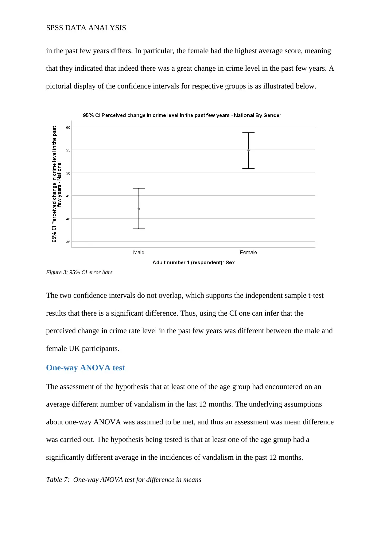
Table 6: Independent sample t-test
Independent Samples Test
Levene's Test for
Equality of
Variances t-test for Equality of Means
F Sig. t df
Sig. (2-
tailed)
Mean
Difference
Std. Error
Difference
95% Confidence Interval
of the Difference
Lower Upper
Perceived
change in crime
level in the past
few years -
National
Equal
variances
assumed
3.929 .048 -4.219 1098 .000 -12.721 3.015 -18.637 -6.805
Equal
variances
not
assumed
-4.223 1040.75
6
.000 -12.721 3.012 -18.633 -6.810
The summary indicates that equal variance assumption is violated (F (1, 1098) = 3.929, p-
value < .05). The t-test for equality of the means shows that there is enough evidence to reject
the null hypothesis. Thus, it can be inferred that male and female perception on crime levels
SPSS DATA ANALYSIS
in the past few years differs. In particular, the female had the highest average score, meaning
that they indicated that indeed there was a great change in crime level in the past few years. A
pictorial display of the confidence intervals for respective groups is as illustrated below.
Figure 3: 95% CI error bars
The two confidence intervals do not overlap, which supports the independent sample t-test
results that there is a significant difference. Thus, using the CI one can infer that the
perceived change in crime rate level in the past few years was different between the male and
female UK participants.
One-way ANOVA test
The assessment of the hypothesis that at least one of the age group had encountered on an
average different number of vandalism in the last 12 months. The underlying assumptions
about one-way ANOVA was assumed to be met, and thus an assessment was mean difference
was carried out. The hypothesis being tested is that at least one of the age group had a
significantly different average in the incidences of vandalism in the past 12 months.
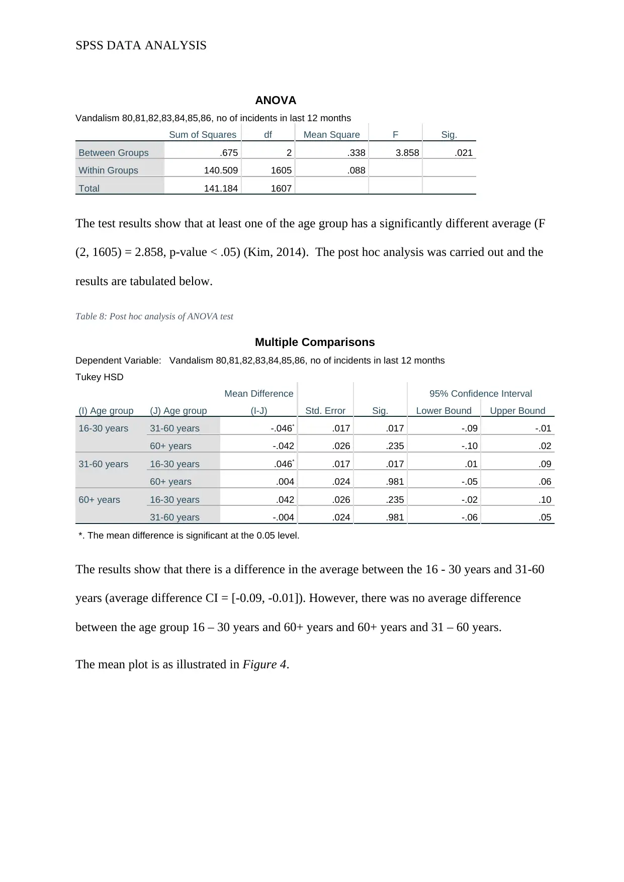
Table 7: One-way ANOVA test for difference in means
SPSS DATA ANALYSIS
ANOVA
Vandalism 80,81,82,83,84,85,86, no of incidents in last 12 months
Sum of Squares df Mean Square F Sig.
Between Groups .675 2 .338 3.858 .021
Within Groups 140.509 1605 .088
Total 141.184 1607
The test results show that at least one of the age group has a significantly different average (F
(2, 1605) = 2.858, p-value < .05) (Kim, 2014). The post hoc analysis was carried out and the
results are tabulated below.
Table 8: Post hoc analysis of ANOVA test
Multiple Comparisons
Dependent Variable: Vandalism 80,81,82,83,84,85,86, no of incidents in last 12 months
Tukey HSD
(I) Age group (J) Age group
Mean Difference
(I-J) Std. Error Sig.
95% Confidence Interval
Lower Bound Upper Bound
16-30 years 31-60 years -.046* .017 .017 -.09 -.01
60+ years -.042 .026 .235 -.10 .02
31-60 years 16-30 years .046* .017 .017 .01 .09
60+ years .004 .024 .981 -.05 .06
60+ years 16-30 years .042 .026 .235 -.02 .10
31-60 years -.004 .024 .981 -.06 .05
*. The mean difference is significant at the 0.05 level.
The results show that there is a difference in the average between the 16 - 30 years and 31-60
years (average difference CI = [-0.09, -0.01]). However, there was no average difference
between the age group 16 – 30 years and 60+ years and 60+ years and 31 – 60 years.
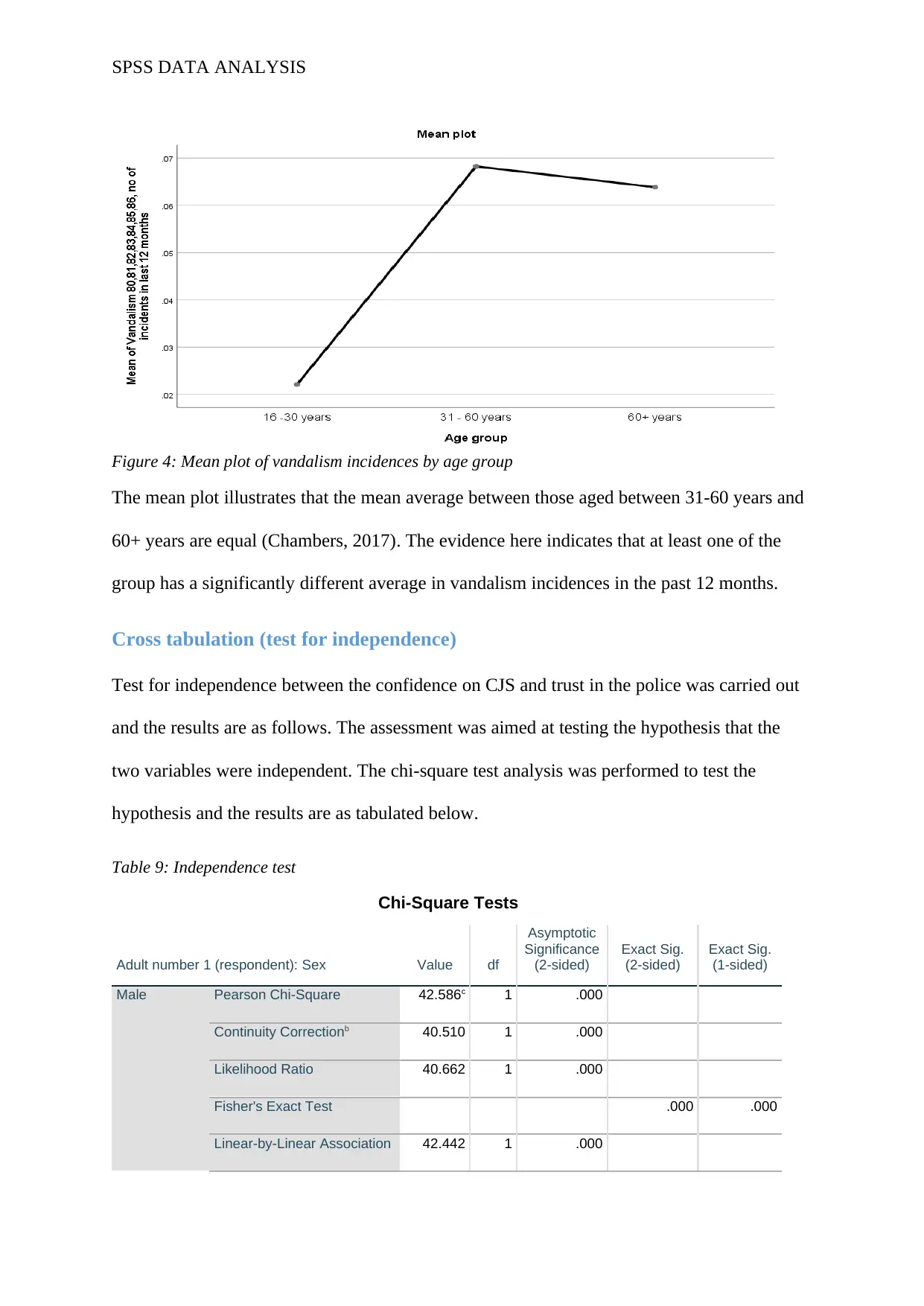
The mean plot is as illustrated in Figure 4.
Secure Best Marks with AI Grader
Need help grading? Try our AI Grader for instant feedback on your assignments.
SPSS DATA ANALYSIS
Figure 4: Mean plot of vandalism incidences by age group
The mean plot illustrates that the mean average between those aged between 31-60 years and
60+ years are equal (Chambers, 2017). The evidence here indicates that at least one of the
group has a significantly different average in vandalism incidences in the past 12 months.
Cross tabulation (test for independence)
Test for independence between the confidence on CJS and trust in the police was carried out
and the results are as follows. The assessment was aimed at testing the hypothesis that the
two variables were independent. The chi-square test analysis was performed to test the
hypothesis and the results are as tabulated below.
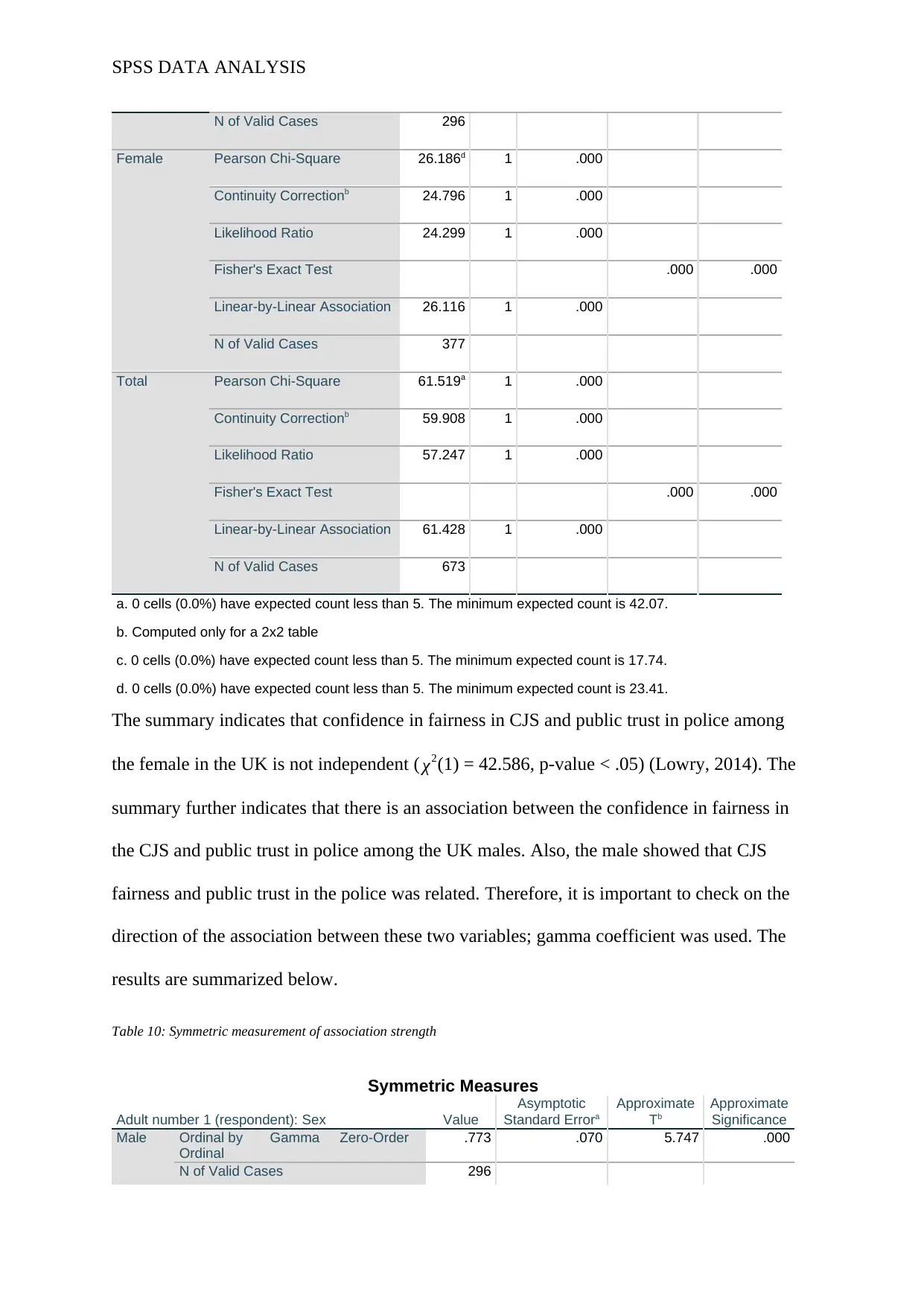
Table 9: Independence test
Chi-Square Tests
Adult number 1 (respondent): Sex Value df
Asymptotic
Significance
(2-sided)
Exact Sig.
(2-sided)
Exact Sig.
(1-sided)
Male Pearson Chi-Square 42.586c 1 .000
Continuity Correctionb 40.510 1 .000
Likelihood Ratio 40.662 1 .000
Fisher's Exact Test .000 .000
Linear-by-Linear Association 42.442 1 .000
SPSS DATA ANALYSIS
N of Valid Cases 296
Female Pearson Chi-Square 26.186d 1 .000
Continuity Correctionb 24.796 1 .000
Likelihood Ratio 24.299 1 .000
Fisher's Exact Test .000 .000
Linear-by-Linear Association 26.116 1 .000
N of Valid Cases 377
Total Pearson Chi-Square 61.519a 1 .000
Continuity Correctionb 59.908 1 .000
Likelihood Ratio 57.247 1 .000
Fisher's Exact Test .000 .000
Linear-by-Linear Association 61.428 1 .000
N of Valid Cases 673
a. 0 cells (0.0%) have expected count less than 5. The minimum expected count is 42.07.
b. Computed only for a 2x2 table
c. 0 cells (0.0%) have expected count less than 5. The minimum expected count is 17.74.
d. 0 cells (0.0%) have expected count less than 5. The minimum expected count is 23.41.
The summary indicates that confidence in fairness in CJS and public trust in police among
the female in the UK is not independent ( χ2(1) = 42.586, p-value < .05) (Lowry, 2014). The
summary further indicates that there is an association between the confidence in fairness in
the CJS and public trust in police among the UK males. Also, the male showed that CJS
fairness and public trust in the police was related. Therefore, it is important to check on the
direction of the association between these two variables; gamma coefficient was used. The
results are summarized below.
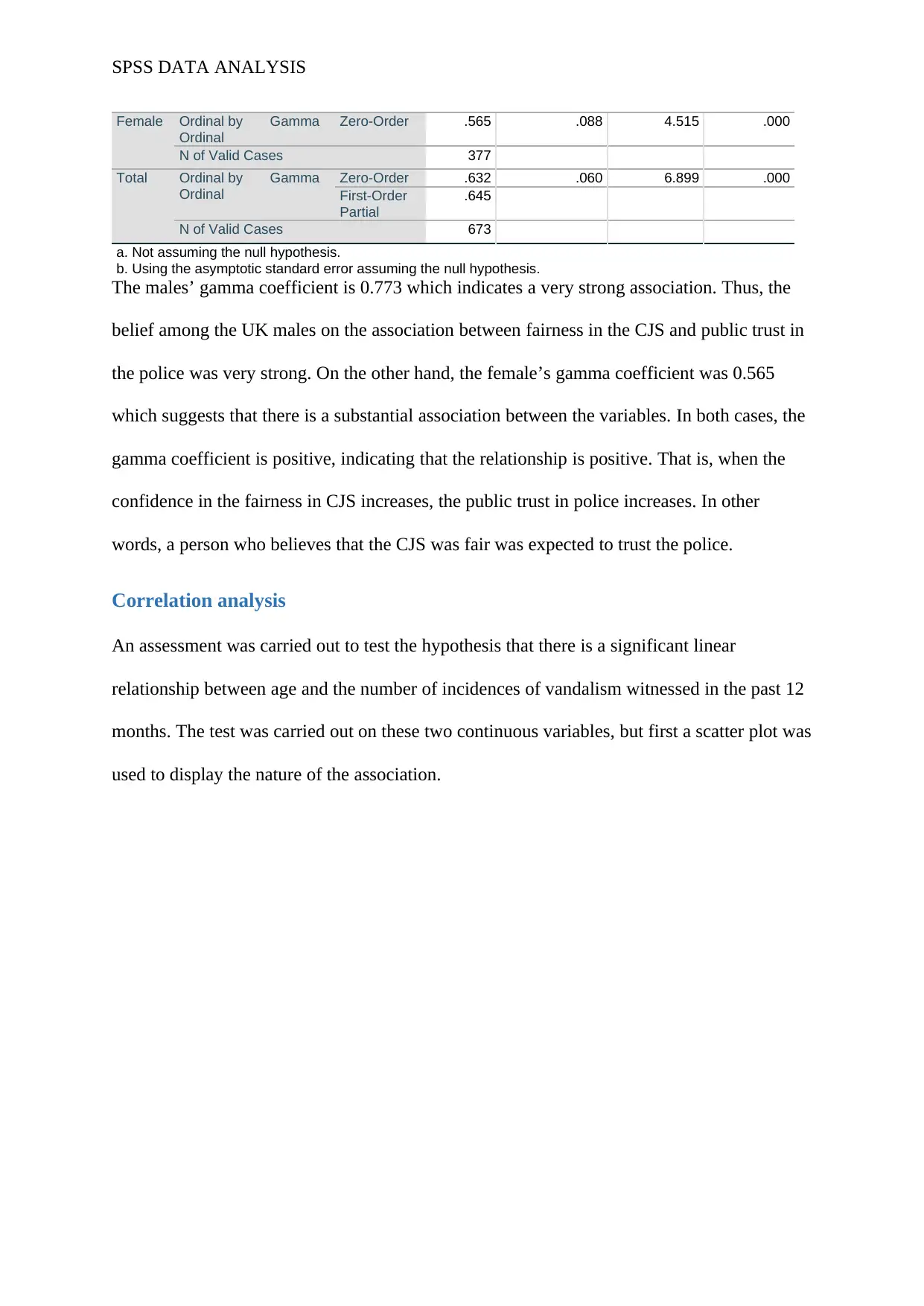
Table 10: Symmetric measurement of association strength
Symmetric Measures
Adult number 1 (respondent): Sex Value
Asymptotic
Standard Errora
Approximate
Tb
Approximate
Significance
Male Ordinal by
Ordinal
Gamma Zero-Order .773 .070 5.747 .000
N of Valid Cases 296
N of Valid Cases 296
Female Pearson Chi-Square 26.186d 1 .000
Continuity Correctionb 24.796 1 .000
Likelihood Ratio 24.299 1 .000
Fisher's Exact Test .000 .000
Linear-by-Linear Association 26.116 1 .000
N of Valid Cases 377
Total Pearson Chi-Square 61.519a 1 .000
Continuity Correctionb 59.908 1 .000
Likelihood Ratio 57.247 1 .000
Fisher's Exact Test .000 .000
Linear-by-Linear Association 61.428 1 .000
N of Valid Cases 673
a. 0 cells (0.0%) have expected count less than 5. The minimum expected count is 42.07.
b. Computed only for a 2x2 table
c. 0 cells (0.0%) have expected count less than 5. The minimum expected count is 17.74.
d. 0 cells (0.0%) have expected count less than 5. The minimum expected count is 23.41.
The summary indicates that confidence in fairness in CJS and public trust in police among
the female in the UK is not independent ( χ2(1) = 42.586, p-value < .05) (Lowry, 2014). The
summary further indicates that there is an association between the confidence in fairness in
the CJS and public trust in police among the UK males. Also, the male showed that CJS
fairness and public trust in the police was related. Therefore, it is important to check on the
direction of the association between these two variables; gamma coefficient was used. The
results are summarized below.
Table 10: Symmetric measurement of association strength
Symmetric Measures
Adult number 1 (respondent): Sex Value
Asymptotic
Standard Errora
Approximate
Tb
Approximate
Significance
Male Ordinal by
Ordinal
Gamma Zero-Order .773 .070 5.747 .000
N of Valid Cases 296
SPSS DATA ANALYSIS
Female Ordinal by
Ordinal
Gamma Zero-Order .565 .088 4.515 .000
N of Valid Cases 377
Total Ordinal by
Ordinal
Gamma Zero-Order .632 .060 6.899 .000
First-Order
Partial
.645
N of Valid Cases 673
a. Not assuming the null hypothesis.
b. Using the asymptotic standard error assuming the null hypothesis.
The males’ gamma coefficient is 0.773 which indicates a very strong association. Thus, the
belief among the UK males on the association between fairness in the CJS and public trust in
the police was very strong. On the other hand, the female’s gamma coefficient was 0.565
which suggests that there is a substantial association between the variables. In both cases, the
gamma coefficient is positive, indicating that the relationship is positive. That is, when the
confidence in the fairness in CJS increases, the public trust in police increases. In other
words, a person who believes that the CJS was fair was expected to trust the police.
Correlation analysis
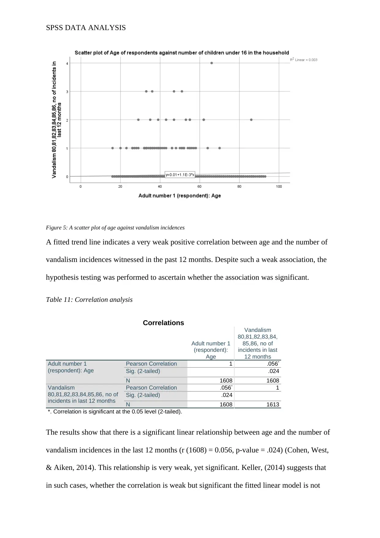
An assessment was carried out to test the hypothesis that there is a significant linear
relationship between age and the number of incidences of vandalism witnessed in the past 12
months. The test was carried out on these two continuous variables, but first a scatter plot was
used to display the nature of the association.
Paraphrase This Document
Need a fresh take? Get an instant paraphrase of this document with our AI Paraphraser
SPSS DATA ANALYSIS
Figure 5: A scatter plot of age against vandalism incidences
A fitted trend line indicates a very weak positive correlation between age and the number of
vandalism incidences witnessed in the past 12 months. Despite such a weak association, the
hypothesis testing was performed to ascertain whether the association was significant.
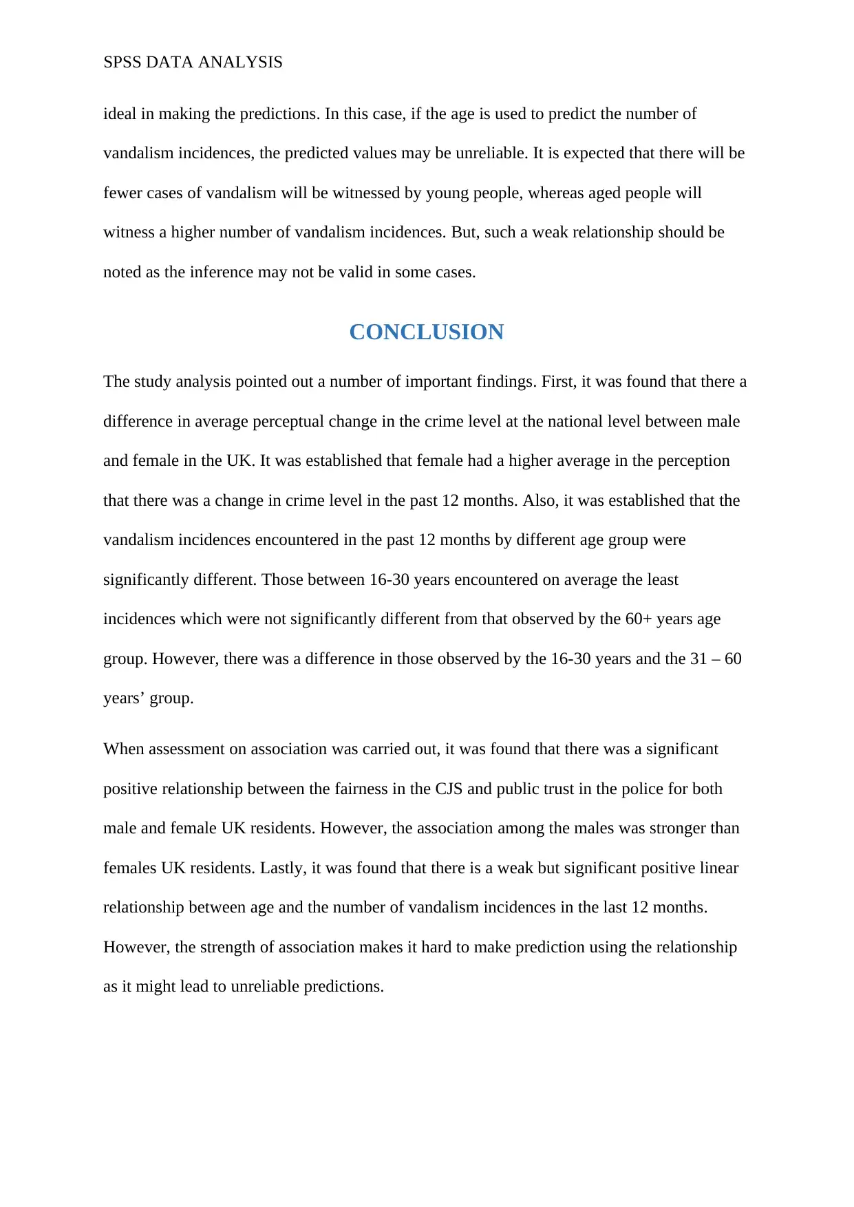
Table 11: Correlation analysis
Correlations
Adult number 1
(respondent):
Age
Vandalism
80,81,82,83,84,
85,86, no of
incidents in last
12 months
Adult number 1
(respondent): Age
Pearson Correlation 1 .056*
Sig. (2-tailed) .024
N 1608 1608
Vandalism
80,81,82,83,84,85,86, no of
incidents in last 12 months
Pearson Correlation .056* 1
Sig. (2-tailed) .024
N 1608 1613
*. Correlation is significant at the 0.05 level (2-tailed).
The results show that there is a significant linear relationship between age and the number of
vandalism incidences in the last 12 months (r (1608) = 0.056, p-value = .024) (Cohen, West,
& Aiken, 2014). This relationship is very weak, yet significant. Keller, (2014) suggests that
in such cases, whether the correlation is weak but significant the fitted linear model is not
SPSS DATA ANALYSIS
ideal in making the predictions. In this case, if the age is used to predict the number of
vandalism incidences, the predicted values may be unreliable. It is expected that there will be
fewer cases of vandalism will be witnessed by young people, whereas aged people will
witness a higher number of vandalism incidences. But, such a weak relationship should be
noted as the inference may not be valid in some cases.
CONCLUSION
The study analysis pointed out a number of important findings. First, it was found that there a
difference in average perceptual change in the crime level at the national level between male
and female in the UK. It was established that female had a higher average in the perception
that there was a change in crime level in the past 12 months. Also, it was established that the
vandalism incidences encountered in the past 12 months by different age group were
significantly different. Those between 16-30 years encountered on average the least
incidences which were not significantly different from that observed by the 60+ years age
group. However, there was a difference in those observed by the 16-30 years and the 31 – 60
years’ group.
When assessment on association was carried out, it was found that there was a significant
positive relationship between the fairness in the CJS and public trust in the police for both
male and female UK residents. However, the association among the males was stronger than
females UK residents. Lastly, it was found that there is a weak but significant positive linear
relationship between age and the number of vandalism incidences in the last 12 months.
However, the strength of association makes it hard to make prediction using the relationship
as it might lead to unreliable predictions.
SPSS DATA ANALYSIS
References
BBC News. (2019, January 24). Crime figures: Violent crime recorded by police rises by
19%. Retrieved from BBC news Services: https://www.bbc.com/news/uk-46984559
Bradford, B., & Myhill, A. (2015). Triggers of change to public confidence in the police and
criminal justice system: Findings from the Crime Survey for England and Wales panel
experiment. Criminology & Criminal Justice, 15(1), 23-43.
Chambers, J. M. (2017). Graphical Methods for Data Analysis: 0. Chapman and Hall/CRC.
Chatfield, C. (2018). Statistics for technology: a course in applied statistics (3rd Edition ed.).
New York: Routledge.
Cohen, P., West, S. G., & Aiken, L. S. (2014). Applied multiple regression/correlation
analysis for the behavioral sciences (2nd ed.). Psychology Press.
Greenberg, D. F. (1985). Age, crime, and social explanation. American journal of sociology,
91(1), 1-21.
Keller, G. (2015). Statistics for Management and Economics, Abbreviated. Cengage
Learning.
Kim, H.-Y. (2014). Analysis of variance (ANOVA) comparing means of more than two
groups. Restorative dentistry & endodontics, 39(1), 74-77.
LaGrange, R. L., & Ferraro, K. F. (2017). The elderly’s fear of crime: A critical examination
of the research. In The fear of crime, 77-96.
Lowry, R. (2014). Concepts and applications of inferential statistics.
Mirrlees-Black, C. (2001). Confidence in the criminal justice system: findings from the 2000
British Crime Survey. London: Home Office.
Secure Best Marks with AI Grader
Need help grading? Try our AI Grader for instant feedback on your assignments.

SPSS DATA ANALYSIS
Park, H. M. (2015). Univariate analysis and normality test using SAS, Stata, and SPSS.
Indiana: IUscholars work.
Roberts, J. (2018). Public opinion, crime, and criminal justice. Routledge.
Sullivan III, M. (2015). Fundamentals of statistics. Pearson.
Thornberry, T. (2018). Developmental theories of crime and delinquency. Routledge.
1 out of 17
Your All-in-One AI-Powered Toolkit for Academic Success.
+13062052269
info@desklib.com
Available 24*7 on WhatsApp / Email
![[object Object]](/_next/static/media/star-bottom.7253800d.svg)
Unlock your academic potential
© 2024 | Zucol Services PVT LTD | All rights reserved.

