SPSS Data Collection - Assignment

Data collection
Data collection is one of the most important part of the every research project. In this case the
data has been collected from 60 different firms which are based on different countries all over
the world. The data was extracted from the master data set using the random sampling method,
which is one of the most popular method for the sample selection. The data set has been provided
in separate excel sheet. The data cleaning process has been completed before importing the data
in the SPSS, such as the removal of the variable which are not required, addressing the missing
values and also coding the variables which are in string form. Results from the data analysis are
discussed in the next section.
Data analysis (Descriptive)
Results from the descriptive statistics helps the researcher to know more about the data in more
meaningful way. The most measures of the descriptive statistics are the median, mode, mean,
variance, standard deviation. Similarly the kurtosis and skewness helps to understand the
distribution of the data.
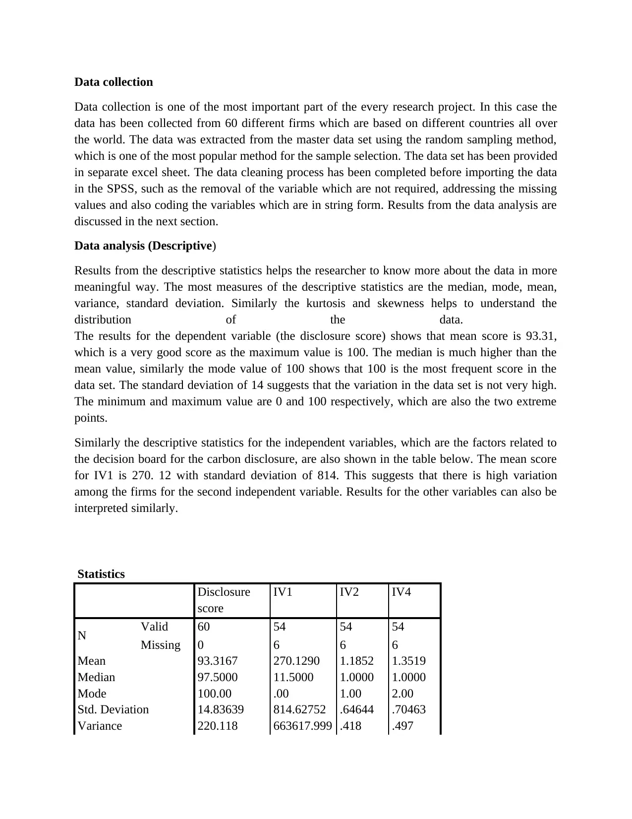
The results for the dependent variable (the disclosure score) shows that mean score is 93.31,
which is a very good score as the maximum value is 100. The median is much higher than the
mean value, similarly the mode value of 100 shows that 100 is the most frequent score in the
data set. The standard deviation of 14 suggests that the variation in the data set is not very high.
The minimum and maximum value are 0 and 100 respectively, which are also the two extreme
points.
Similarly the descriptive statistics for the independent variables, which are the factors related to
the decision board for the carbon disclosure, are also shown in the table below. The mean score
for IV1 is 270. 12 with standard deviation of 814. This suggests that there is high variation
among the firms for the second independent variable. Results for the other variables can also be
interpreted similarly.
Statistics
Disclosure
score
IV1 IV2 IV4
N Valid 60 54 54 54
Missing 0 6 6 6
Mean 93.3167 270.1290 1.1852 1.3519
Median 97.5000 11.5000 1.0000 1.0000
Mode 100.00 .00 1.00 2.00
Std. Deviation 14.83639 814.62752 .64644 .70463
Variance 220.118 663617.999 .418 .497

Skewness -4.820 3.913 -.192 -.623
Std. Error of
Skewness
.309 .325 .325 .325
Kurtosis 27.344 15.472 -.595 -.753
Std. Error of Kurtosis .608 .639 .639 .639
Minimum .00 .00 .00 .00
Maximum 100.00 3981.00 2.00 2.00
Percentiles
25 94.0000 .0293 1.0000 1.0000
50 97.5000 11.5000 1.0000 1.0000
75 99.7500 74.0750 2.0000 2.0000
Histograms

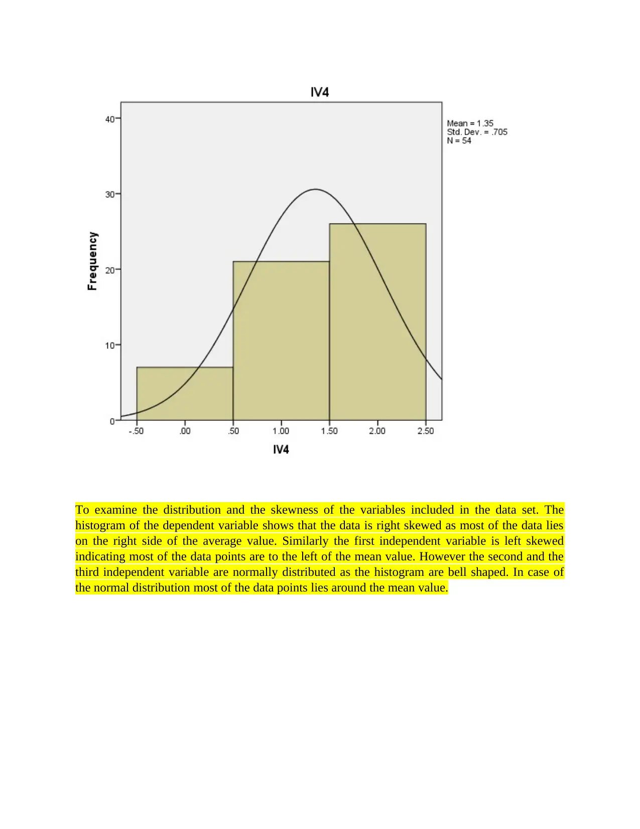
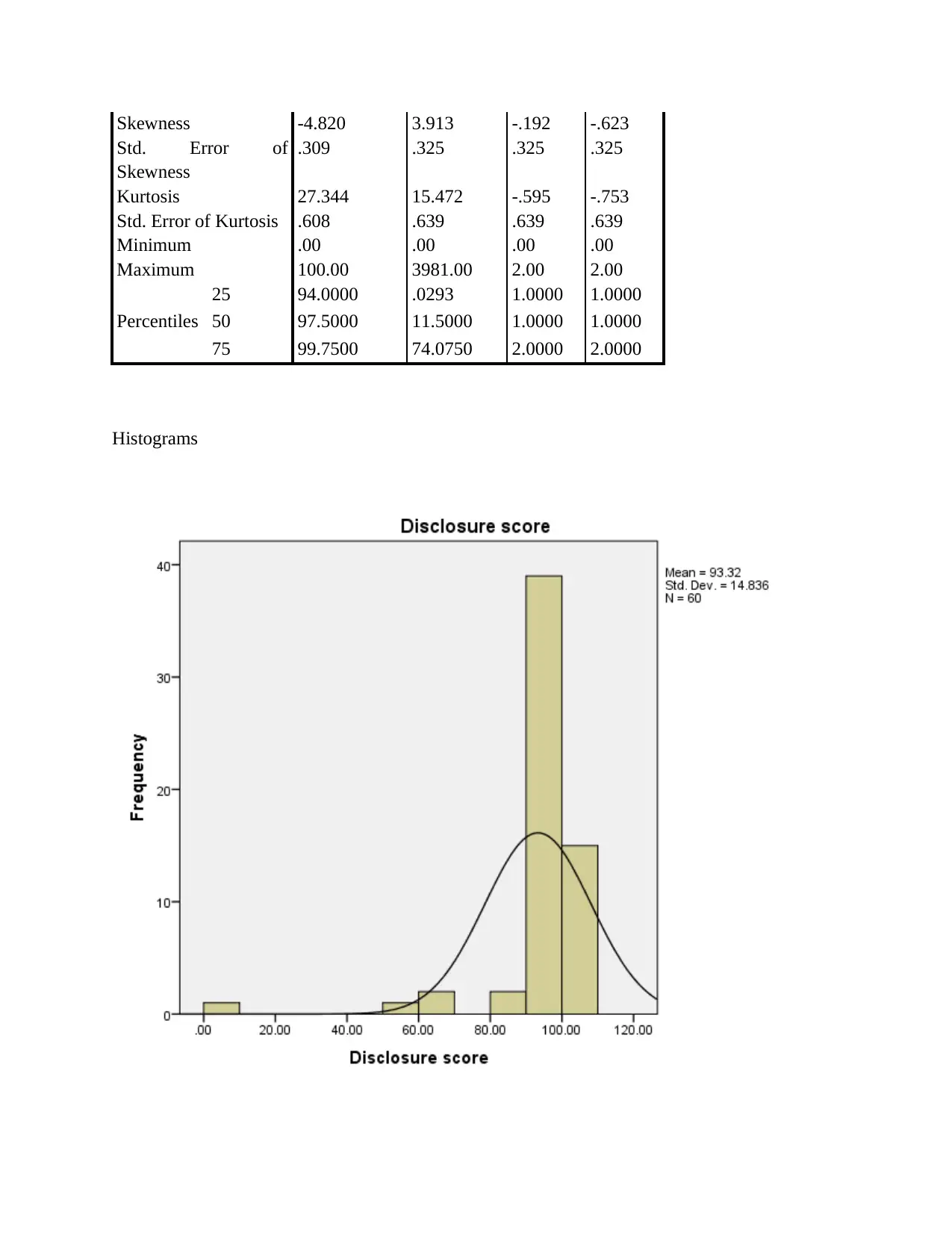
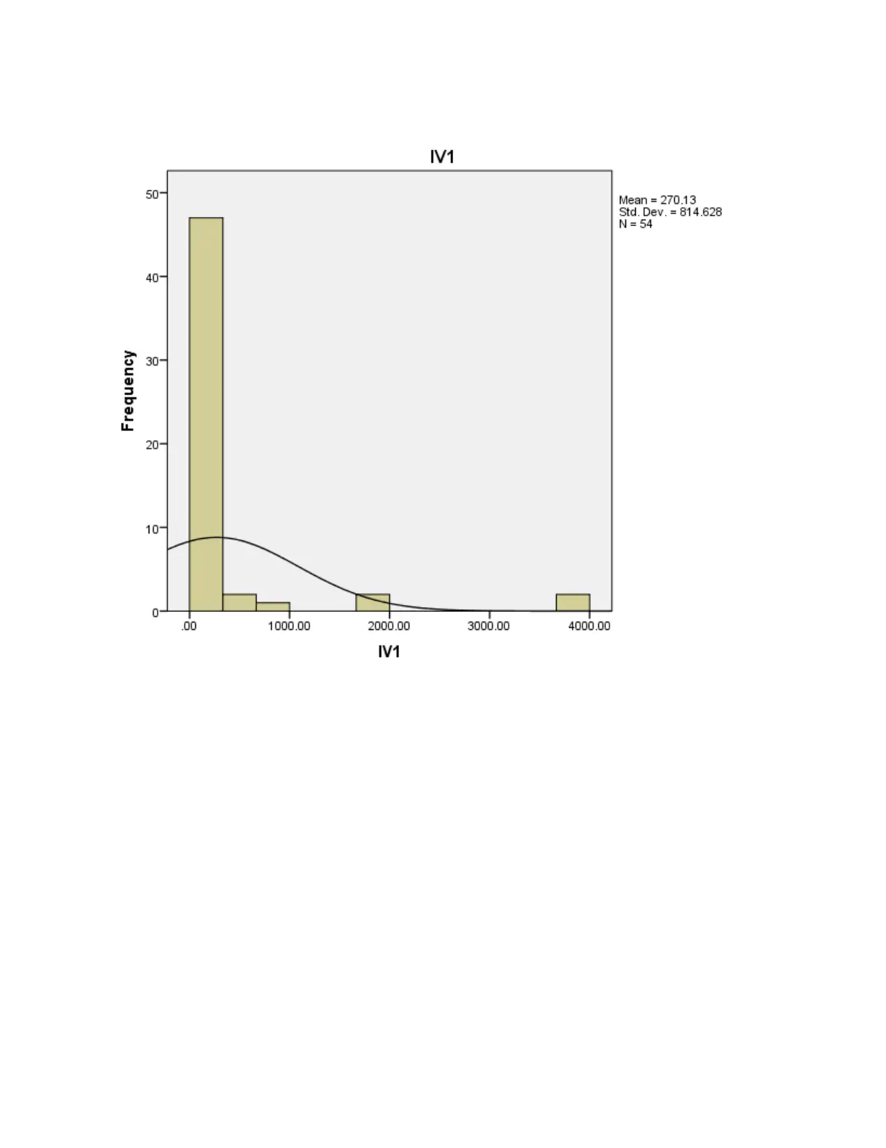
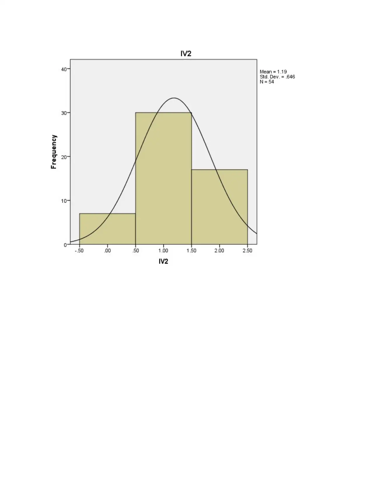
To examine the distribution and the skewness of the variables included in the data set. The
histogram of the dependent variable shows that the data is right skewed as most of the data lies
on the right side of the average value. Similarly the first independent variable is left skewed
indicating most of the data points are to the left of the mean value. However the second and the
third independent variable are normally distributed as the histogram are bell shaped. In case of
the normal distribution most of the data points lies around the mean value.

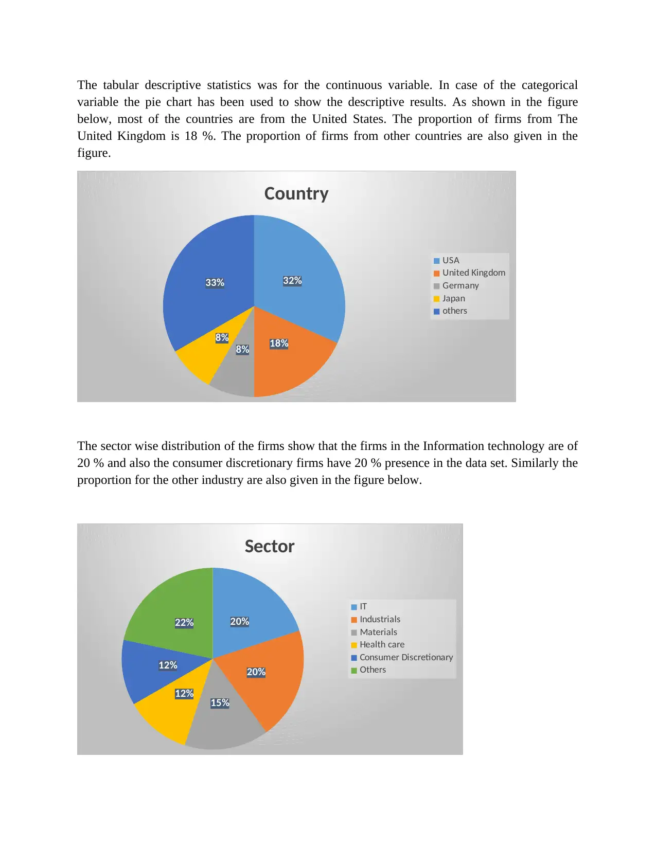
The tabular descriptive statistics was for the continuous variable. In case of the categorical
variable the pie chart has been used to show the descriptive results. As shown in the figure
below, most of the countries are from the United States. The proportion of firms from The
United Kingdom is 18 %. The proportion of firms from other countries are also given in the
figure.
32%
18%
8%
8%
33%
Country
USA
United Kingdom
Germany
Japan
others
The sector wise distribution of the firms show that the firms in the Information technology are of
20 % and also the consumer discretionary firms have 20 % presence in the data set. Similarly the
proportion for the other industry are also given in the figure below.
20%
20%
15%
12%
12%
22%
Sector
IT
Industrials
Materials
Health care
Consumer Discretionary
Others

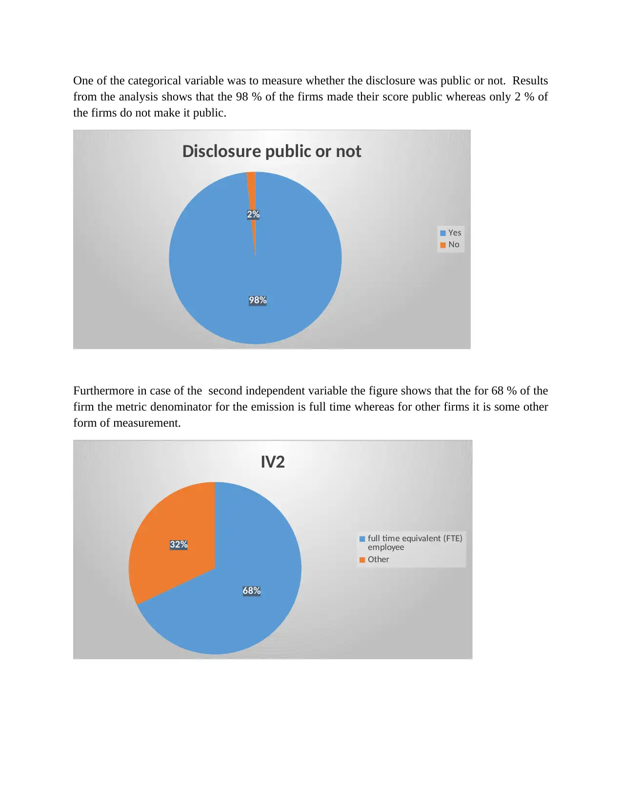
One of the categorical variable was to measure whether the disclosure was public or not. Results
from the analysis shows that the 98 % of the firms made their score public whereas only 2 % of
the firms do not make it public.
98%
2%
Disclosure public or not
Yes
No
Furthermore in case of the second independent variable the figure shows that the for 68 % of the
firm the metric denominator for the emission is full time whereas for other firms it is some other
form of measurement.
68%
32%
IV2
full time equivalent (FTE)
employee
Other

Data analysis (inferential)
This section is devoted to the inferential analysis for the current research paper. Inferential
analysis are used to test the hypothesis which are proposed by the researcher at the beginning of
the project. In this case also the inferential analysis has been conducted using the chi square test,
correlation analysis and the regression analysis.
Country
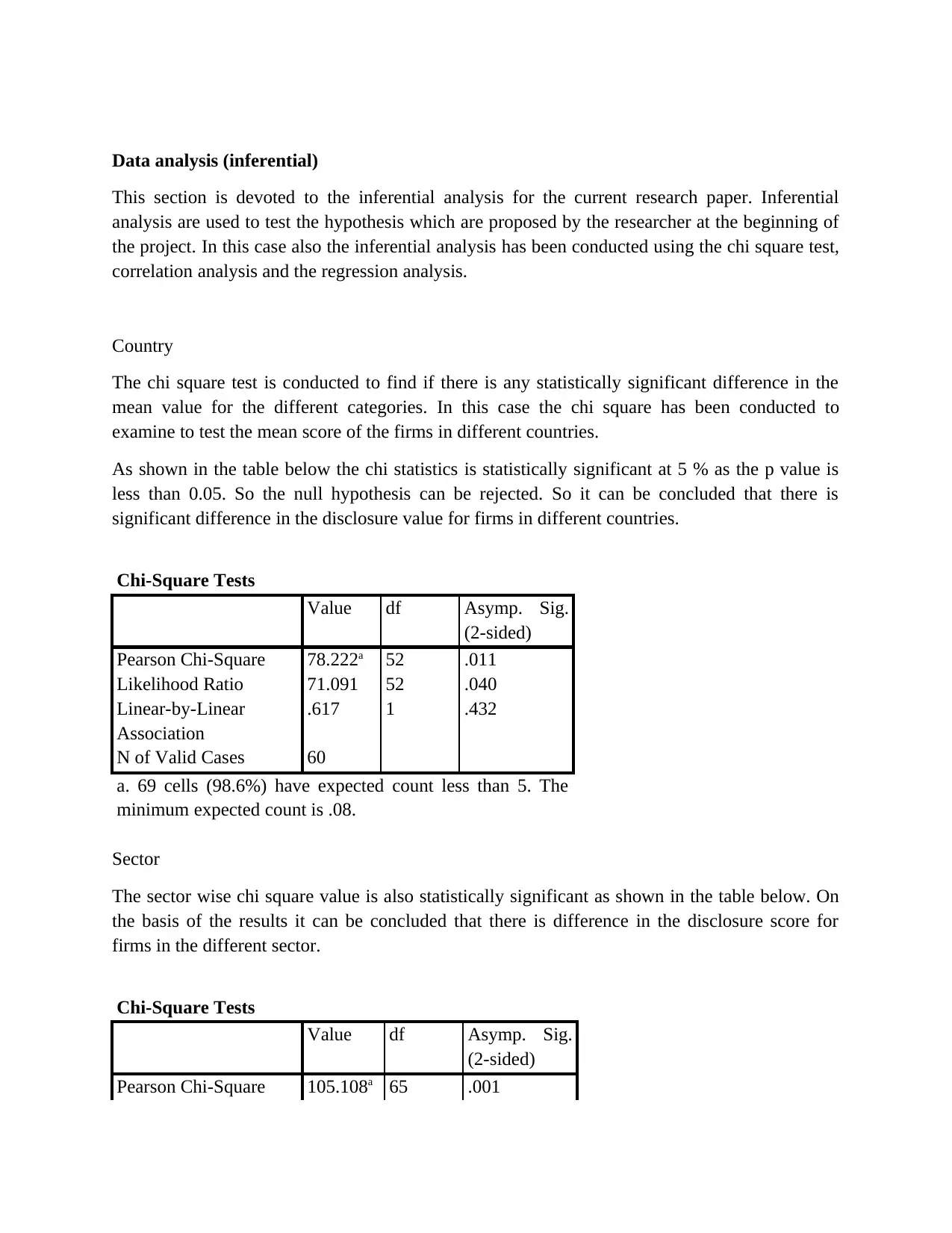
The chi square test is conducted to find if there is any statistically significant difference in the
mean value for the different categories. In this case the chi square has been conducted to
examine to test the mean score of the firms in different countries.
As shown in the table below the chi statistics is statistically significant at 5 % as the p value is
less than 0.05. So the null hypothesis can be rejected. So it can be concluded that there is
significant difference in the disclosure value for firms in different countries.
Chi-Square Tests
Value df Asymp. Sig.
(2-sided)
Pearson Chi-Square 78.222a 52 .011
Likelihood Ratio 71.091 52 .040
Linear-by-Linear
Association
.617 1 .432
N of Valid Cases 60
a. 69 cells (98.6%) have expected count less than 5. The
minimum expected count is .08.
Sector
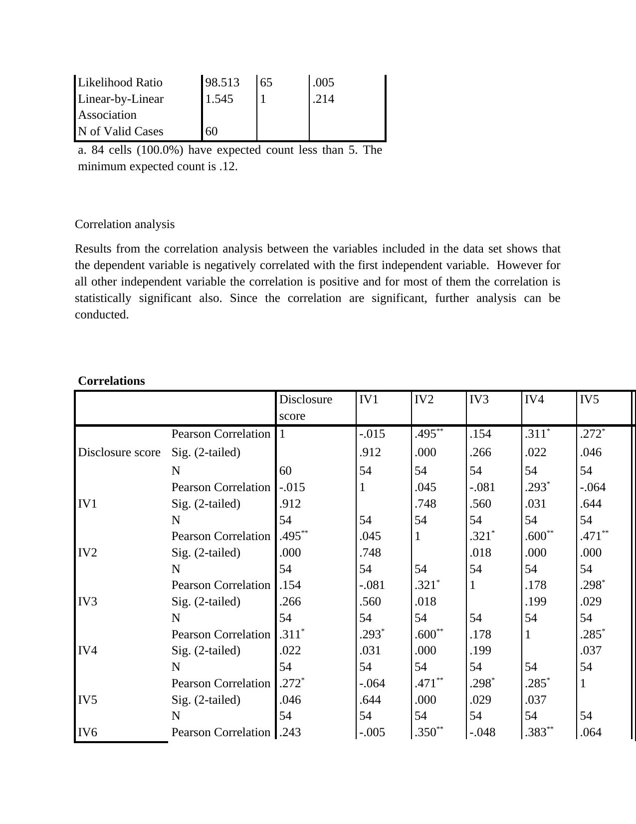
The sector wise chi square value is also statistically significant as shown in the table below. On
the basis of the results it can be concluded that there is difference in the disclosure score for
firms in the different sector.
Chi-Square Tests
Value df Asymp. Sig.
(2-sided)
Pearson Chi-Square 105.108a 65 .001

Likelihood Ratio 98.513 65 .005
Linear-by-Linear
Association
1.545 1 .214
N of Valid Cases 60
a. 84 cells (100.0%) have expected count less than 5. The
minimum expected count is .12.
Correlation analysis
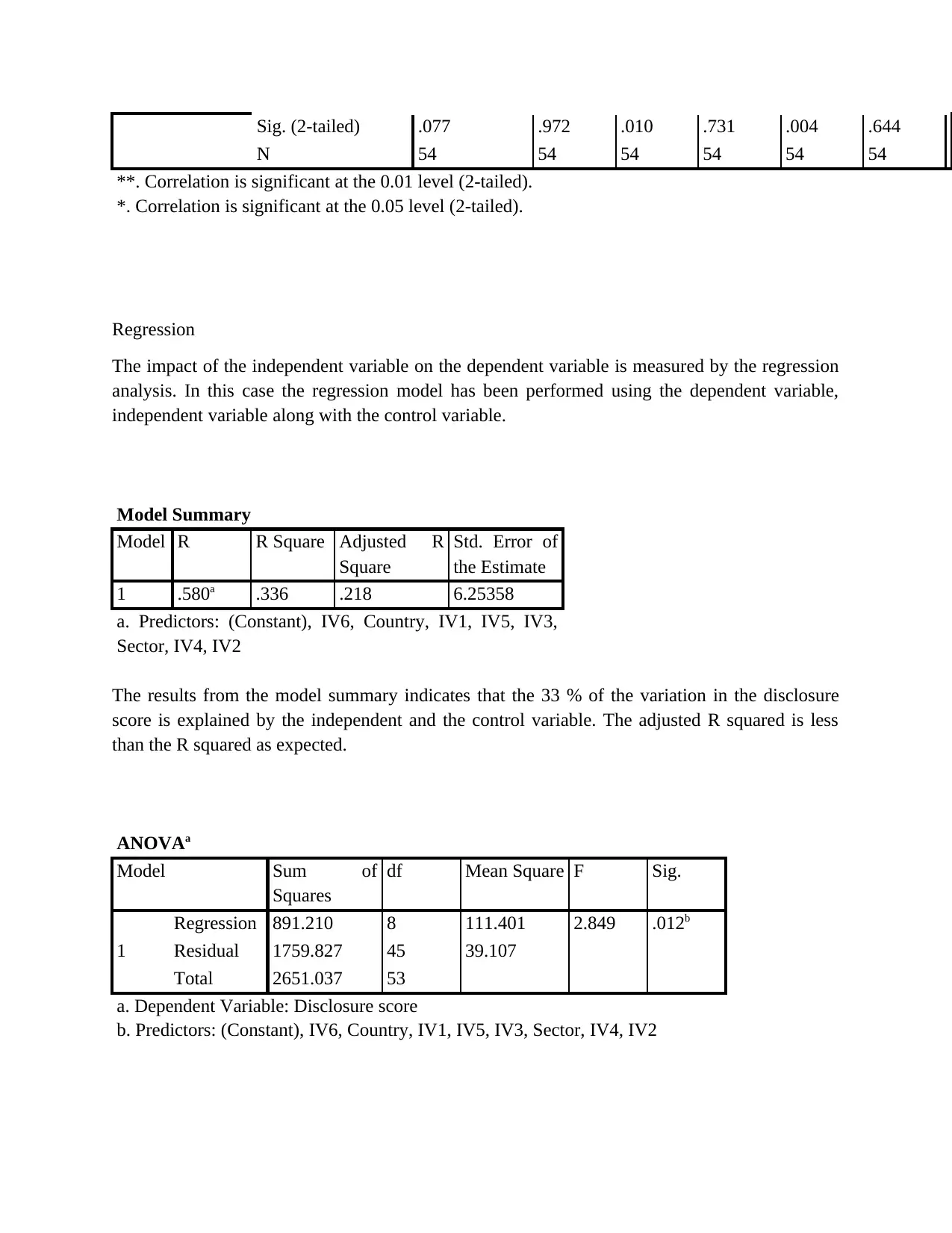
Results from the correlation analysis between the variables included in the data set shows that
the dependent variable is negatively correlated with the first independent variable. However for
all other independent variable the correlation is positive and for most of them the correlation is
statistically significant also. Since the correlation are significant, further analysis can be
conducted.
Correlations
Disclosure
score
IV1 IV2 IV3 IV4 IV5 I
Disclosure score
Pearson Correlation 1 -.015 .495** .154 .311* .272* .
Sig. (2-tailed) .912 .000 .266 .022 .046 .
N 60 54 54 54 54 54 5
IV1
Pearson Correlation -.015 1 .045 -.081 .293* -.064 -
Sig. (2-tailed) .912 .748 .560 .031 .644 .
N 54 54 54 54 54 54 5
IV2
Pearson Correlation .495** .045 1 .321* .600** .471** .
Sig. (2-tailed) .000 .748 .018 .000 .000 .
N 54 54 54 54 54 54 5
IV3
Pearson Correlation .154 -.081 .321* 1 .178 .298* -
Sig. (2-tailed) .266 .560 .018 .199 .029 .
N 54 54 54 54 54 54 5
IV4
Pearson Correlation .311* .293* .600** .178 1 .285* .
Sig. (2-tailed) .022 .031 .000 .199 .037 .
N 54 54 54 54 54 54 5
IV5
Pearson Correlation .272* -.064 .471** .298* .285* 1 .
Sig. (2-tailed) .046 .644 .000 .029 .037 .
N 54 54 54 54 54 54 5
IV6 Pearson Correlation .243 -.005 .350** -.048 .383** .064 1

Sig. (2-tailed) .077 .972 .010 .731 .004 .644
N 54 54 54 54 54 54 5
**. Correlation is significant at the 0.01 level (2-tailed).
*. Correlation is significant at the 0.05 level (2-tailed).
Regression
The impact of the independent variable on the dependent variable is measured by the regression
analysis. In this case the regression model has been performed using the dependent variable,
independent variable along with the control variable.
Model Summary
Model R R Square Adjusted R
Square
Std. Error of
the Estimate
1 .580a .336 .218 6.25358
a. Predictors: (Constant), IV6, Country, IV1, IV5, IV3,
Sector, IV4, IV2
The results from the model summary indicates that the 33 % of the variation in the disclosure
score is explained by the independent and the control variable. The adjusted R squared is less
than the R squared as expected.
ANOVAa
Model Sum of
Squares
df Mean Square F Sig.
1
Regression 891.210 8 111.401 2.849 .012b
Residual 1759.827 45 39.107
Total 2651.037 53
a. Dependent Variable: Disclosure score
b. Predictors: (Constant), IV6, Country, IV1, IV5, IV3, Sector, IV4, IV2

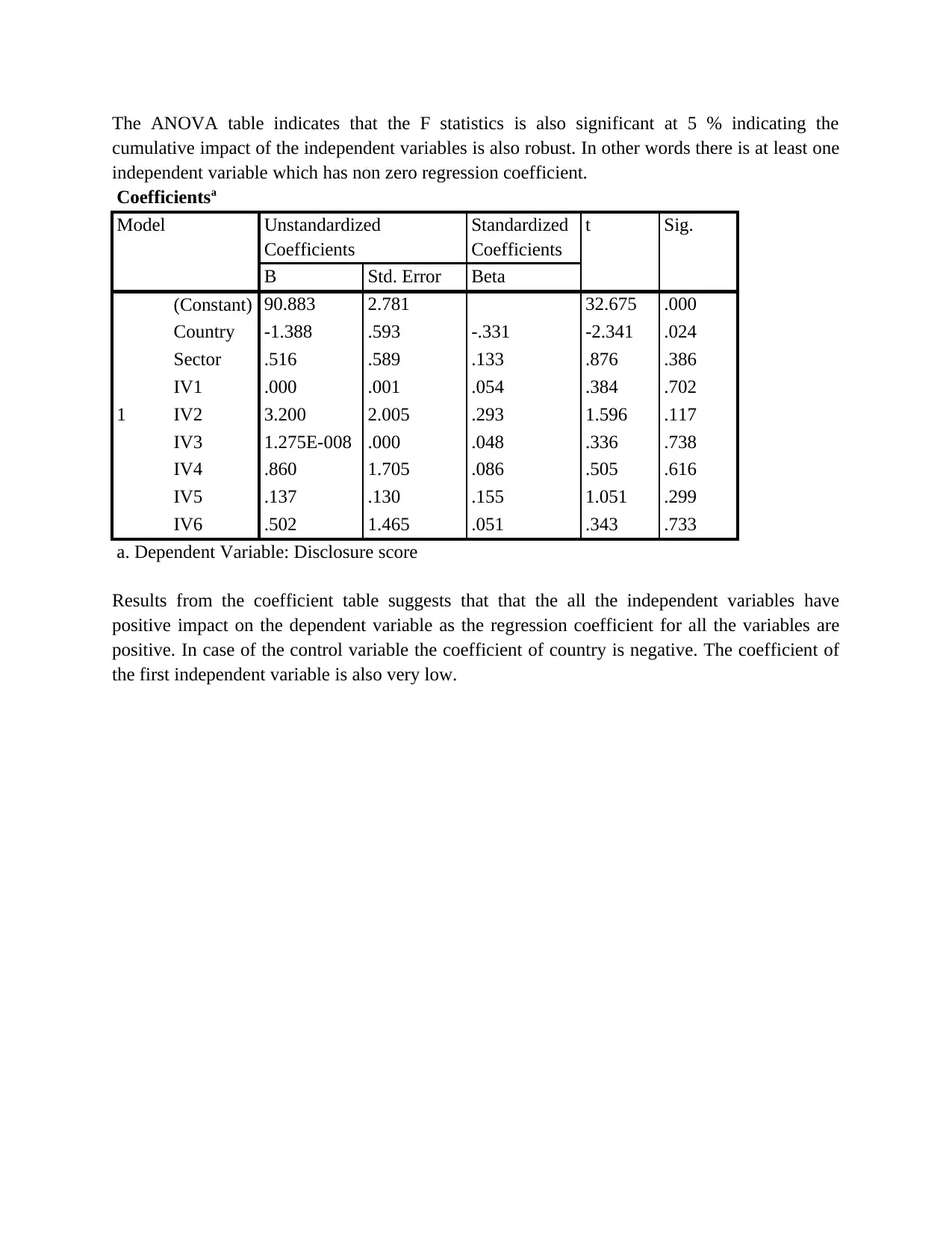
The ANOVA table indicates that the F statistics is also significant at 5 % indicating the
cumulative impact of the independent variables is also robust. In other words there is at least one
independent variable which has non zero regression coefficient.
Coefficientsa
Model Unstandardized
Coefficients
Standardized
Coefficients
t Sig.
B Std. Error Beta
1
(Constant) 90.883 2.781 32.675 .000
Country -1.388 .593 -.331 -2.341 .024
Sector .516 .589 .133 .876 .386
IV1 .000 .001 .054 .384 .702
IV2 3.200 2.005 .293 1.596 .117
IV3 1.275E-008 .000 .048 .336 .738
IV4 .860 1.705 .086 .505 .616
IV5 .137 .130 .155 1.051 .299
IV6 .502 1.465 .051 .343 .733
a. Dependent Variable: Disclosure score
Results from the coefficient table suggests that that the all the independent variables have
positive impact on the dependent variable as the regression coefficient for all the variables are
positive. In case of the control variable the coefficient of country is negative. The coefficient of
the first independent variable is also very low.