SPSS practice project

This document provides a practice project on SPSS, covering topics such as common bias test, univariate statistics, reliability testing, correlation tests, t-test analysis, and more. It includes descriptive statistics, case processing summary, reliability statistics, correlation results, and t-test analysis. The document is suitable for students studying SPSS or conducting research using SPSS software.

SPSS practice project

Contents
1. Common bias test....................................................................................................................1
2. Univariate statistics..................................................................................................................1
3. Reliability testing.....................................................................................................................2
4. Correlation tests.......................................................................................................................2
5. t-test analysis...........................................................................................................................3
6. Chi-square test.........................................................................................................................8
7. The ANOVA tests....................................................................................................................8
8. Linear/multiple regression tests.............................................................................................11
9. Factor analysis and confirmatory tests..................................................................................12

1. Common bias test
A common bias test is a process of check the responses for common bias. The concept of
common bias is a situation when variations or bias in responses are caused due to instruments
which lead to result contamination by the “noise”. In order to ensure that the responses which are
gained from respondents are free from any bias and noise, the common bias test is used.
2. Univariate statistics
Descriptive Statistics
N Minimum Maximum Mean Std. Deviation
C3-V1 192 2 5 4.80 .496
C3-V2 192 0 5 4.39 .744
C1-V3 192 0 5 4.11 .942
C1-V4 192 0 5 4.03 .903
C1-V5 192 0 5 4.04 .912
C1-V6 192 0 5 3.89 1.020
C1-V7 192 0 5 2.91 1.281
C1-V8 192 0 5 3.42 1.137
C1-V9 192 0 5 3.79 .914
C1-V10 192 0 5 3.34 1.169
C3-V11 192 0 5 3.64 1.064
C3-V12 192 0 5 3.62 .963
C3-V13 192 0 5 3.49 1.054
C3-V14 192 0 5 3.46 1.171
C3-V15 192 0 5 2.66 1.247
C3-V16 192 0 5 2.96 1.240
C2-V17 192 0 5 3.13 1.130
C2-V18 192 0 5 3.56 1.086
C2-V19 192 0 5 3.08 1.316
C2-V20 192 0 5 3.19 1.147
C1-V21 192 0 5 3.35 1.179
C2-V22 192 0 5 3.15 1.145
C2-V23 192 0 5 3.22 1.247
Gender 192 0 1 .43 .496
Position Class 192 0 6 2.83 1.550
Employee Evaluation 192 0 5 3.51 1.483
1

Valid N (listwise) 192
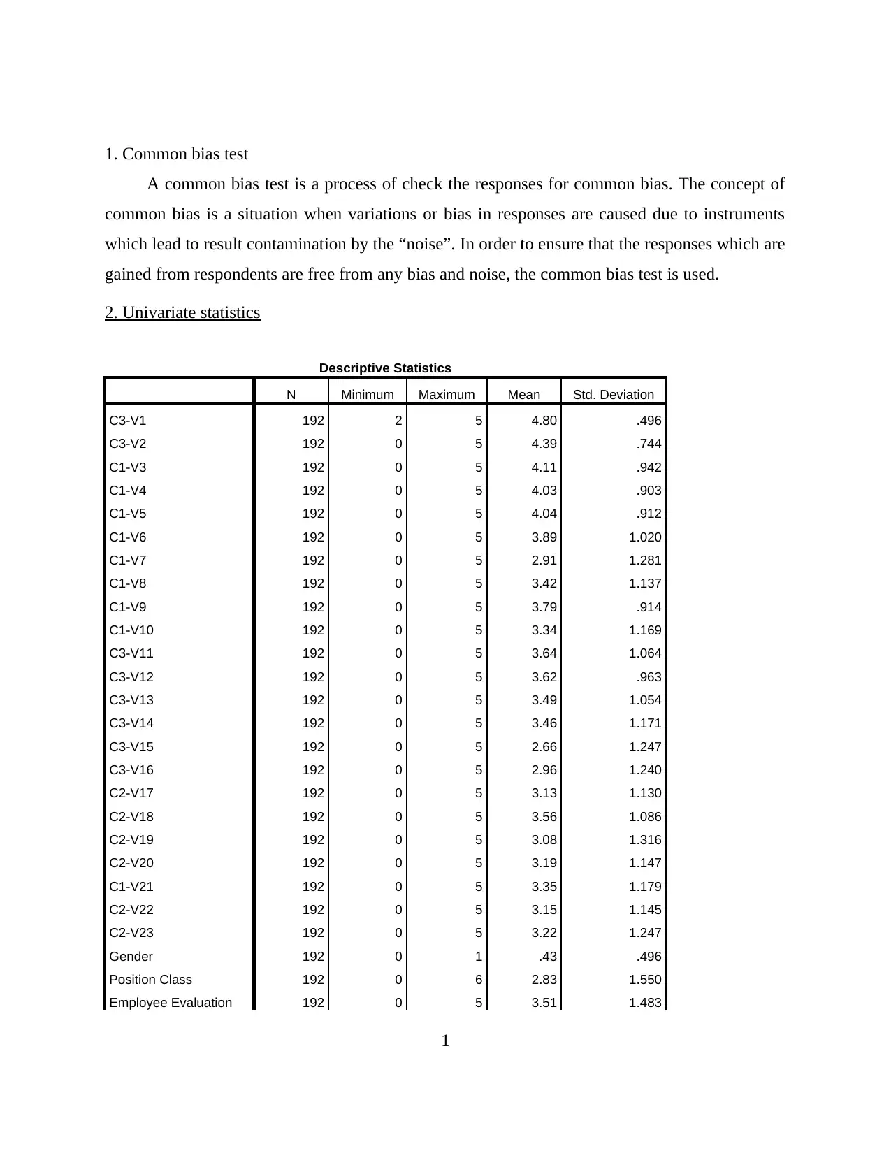
Using the lab data given, descriptive of all the variables of the data set are calculated using
SPSS. The above data shows three categorical variables which are considered as independent and
various dependent variables (from C3-V1 to C2-V23). Descriptive statistics including mean,
minimum, maximum and standard deviation is calculated for every variable. For example the
variable C3-V1 shows that the total number of respondents are 192, the mean response of every
respondent is 4.80 with standard variation of .496. The minimum value of the response is 2 and
maximum is 5.
3. Reliability testing
Case Processing Summary
N %
Cases Valid 192 100.0
Excludeda 0 .0
Total 192 100.0
a. Listwise deletion based on all variables in the
procedure.
Reliability Statistics
Cronbach's
Alpha N of Items
.842 26
A reliability testing is a common procedure from which reliability of the responses or of
data can be measured. The purpose of conducting a reliability test is to study the measurement
scales so that it can provide information about the relationship between the scales.
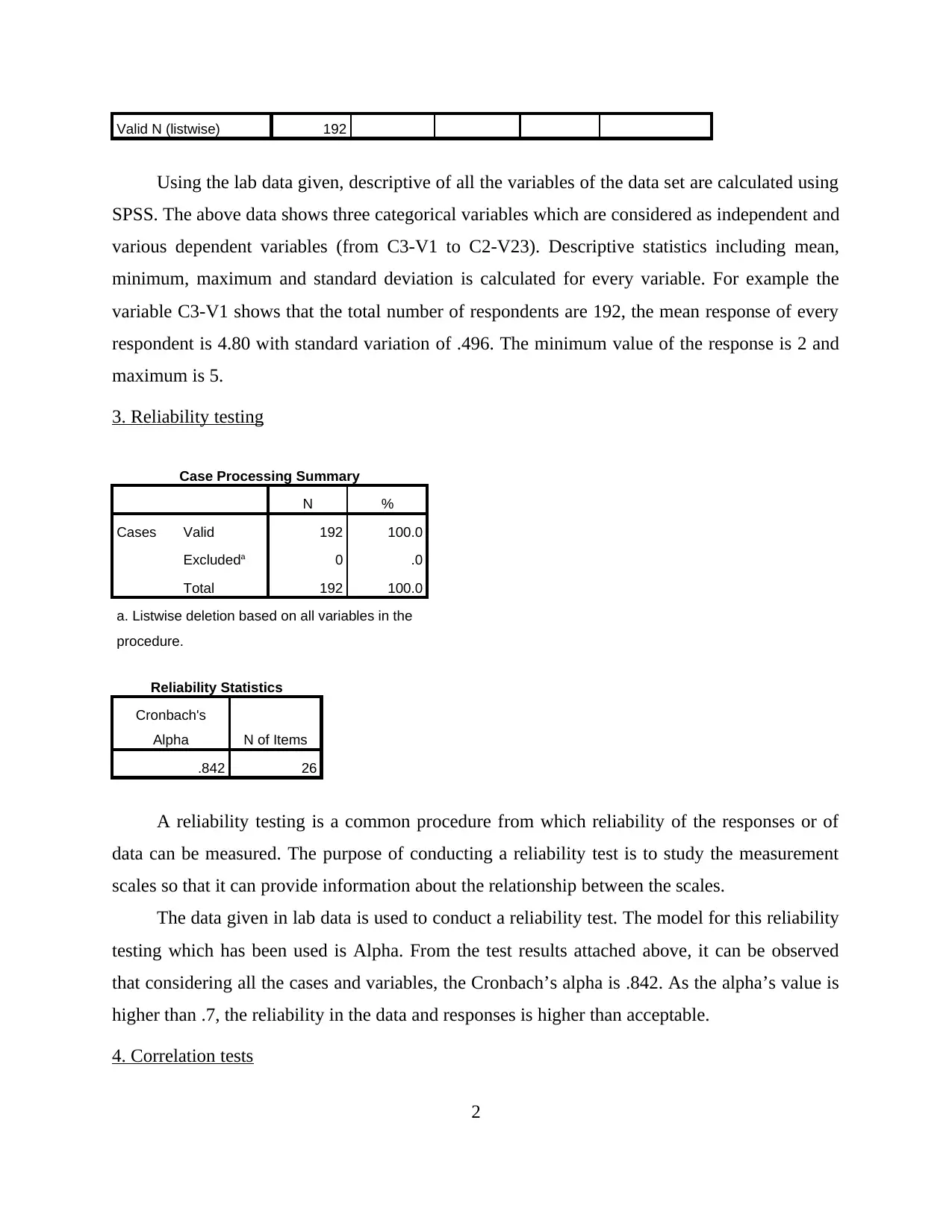
The data given in lab data is used to conduct a reliability test. The model for this reliability
testing which has been used is Alpha. From the test results attached above, it can be observed
that considering all the cases and variables, the Cronbach’s alpha is .842. As the alpha’s value is
higher than .7, the reliability in the data and responses is higher than acceptable.
4. Correlation tests
2

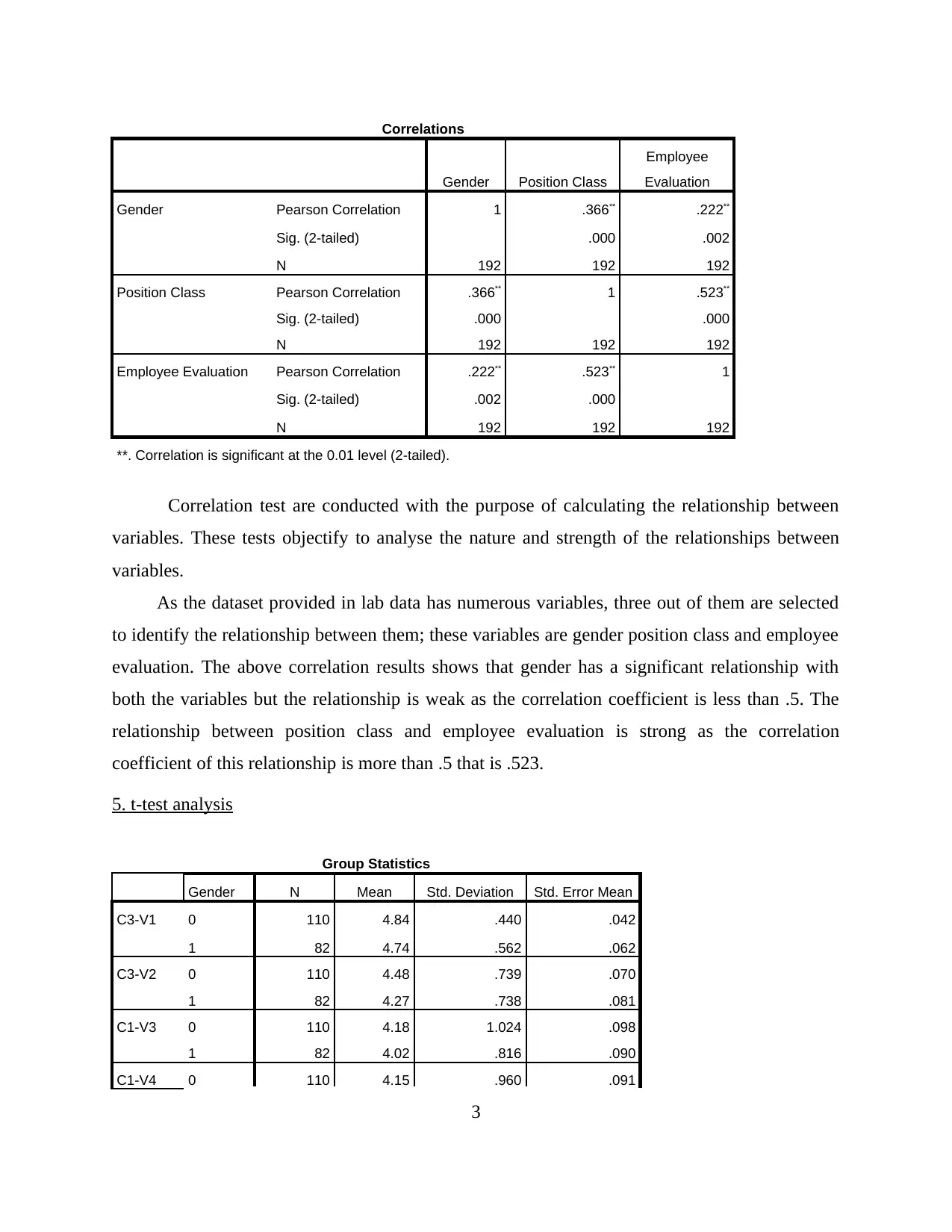
Correlations
Gender Position Class
Employee
Evaluation
Gender Pearson Correlation 1 .366** .222**
Sig. (2-tailed) .000 .002
N 192 192 192
Position Class Pearson Correlation .366** 1 .523**
Sig. (2-tailed) .000 .000
N 192 192 192
Employee Evaluation Pearson Correlation .222** .523** 1
Sig. (2-tailed) .002 .000
N 192 192 192
**. Correlation is significant at the 0.01 level (2-tailed).
Correlation test are conducted with the purpose of calculating the relationship between
variables. These tests objectify to analyse the nature and strength of the relationships between
variables.
As the dataset provided in lab data has numerous variables, three out of them are selected
to identify the relationship between them; these variables are gender position class and employee
evaluation. The above correlation results shows that gender has a significant relationship with
both the variables but the relationship is weak as the correlation coefficient is less than .5. The
relationship between position class and employee evaluation is strong as the correlation
coefficient of this relationship is more than .5 that is .523.
5. t-test analysis
Group Statistics
Gender N Mean Std. Deviation Std. Error Mean
C3-V1 0 110 4.84 .440 .042
1 82 4.74 .562 .062
C3-V2 0 110 4.48 .739 .070
1 82 4.27 .738 .081
C1-V3 0 110 4.18 1.024 .098
1 82 4.02 .816 .090
C1-V4 0 110 4.15 .960 .091
3

1 82 3.87 .798 .088
C1-V5 0 110 4.05 1.012 .097
1 82 4.01 .762 .084
C1-V6 0 110 3.92 1.142 .109
1 82 3.85 .833 .092
C1-V7 0 110 3.15 1.363 .130
1 82 2.59 1.088 .120
C1-V8 0 110 3.55 1.130 .108
1 82 3.26 1.131 .125
C1-V9 0 110 3.82 .988 .094
1 82 3.76 .810 .089
C1-V10 0 110 3.35 1.208 .115
1 82 3.32 1.121 .124
C3-V11 0 110 3.50 1.139 .109
1 82 3.83 .927 .102
C3-V12 0 110 3.59 1.007 .096
1 82 3.66 .906 .100
C3-V13 0 110 3.45 1.138 .109
1 82 3.55 .932 .103
C3-V14 0 110 3.53 1.186 .113
1 82 3.38 1.151 .127
C3-V15 0 110 2.73 1.313 .125
1 82 2.57 1.155 .128
C3-V16 0 110 2.89 1.323 .126
1 82 3.05 1.121 .124
C2-V17 0 110 3.08 1.279 .122
1 82 3.20 .895 .099
C2-V18 0 110 3.61 1.197 .114
1 82 3.50 .920 .102
C2-V19 0 110 3.02 1.453 .138
1 82 3.17 1.109 .122
C2-V20 0 110 3.23 1.232 .117
1 82 3.13 1.028 .113
C1-V21 0 110 3.45 1.170 .112
1 82 3.22 1.187 .131
C2-V22 0 110 3.22 1.207 .115
1 82 3.06 1.058 .117
4

C2-V23 0 110 3.09 1.267 .121
1 82 3.39 1.204 .133
Independent Samples Test
Levene's Test for
Equality of
Variances t-test for Equality of Means
F Sig. t df
Sig. (2-
tailed)
Mean
Difference
Std. Error
Difference
95% Confidence
Interval of the
Difference
Lower Upper
C3-
V1
Equal variances
assumed 5.802 .017 1.279 190 .203 .092 .072 -.050 .235
Equal variances
not assumed 1.234 148.640 .219 .092 .075 -.056 .241
C3-
V2
Equal variances
assumed .045 .832 1.982 190 .049 .214 .108 .001 .426
Equal variances
not assumed 1.983 174.749 .049 .214 .108 .001 .426
C1-
V3
Equal variances
assumed 7.207 .008 1.146 190 .253 .157 .137 -.113 .428
Equal variances
not assumed 1.185 189.126 .238 .157 .133 -.105 .420
C1-
V4
Equal variances
assumed .981 .323 2.213 190 .028 .289 .130 .031 .546
Equal variances
not assumed 2.273 187.708 .024 .289 .127 .038 .539
C1-
V5
Equal variances
assumed 4.386 .038 .318 190 .751 .042 .133 -.221 .305
Equal variances
not assumed .331 189.978 .741 .042 .128 -.210 .295
C1-
V6
Equal variances
assumed 2.643 .106 .433 190 .666 .065 .149 -.230 .359
Equal variances
not assumed .452 189.925 .651 .065 .143 -.217 .346
5

C1-
V7
Equal variances
assumed 6.335 .013 3.114 190 .002 .569 .183 .209 .930
Equal variances
not assumed 3.216 189.067 .002 .569 .177 .220 .918
C1-
V8
Equal variances
assumed .053 .819 1.754 190 .081 .289 .165 -.036 .615
Equal variances
not assumed 1.754 174.595 .081 .289 .165 -.036 .615
C1-
V9
Equal variances
assumed 1.920 .167 .464 190 .643 .062 .134 -.202 .326
Equal variances
not assumed .478 188.241 .633 .062 .130 -.194 .318
C1-
V10
Equal variances
assumed .662 .417 .219 190 .827 .037 .171 -.300 .375
Equal variances
not assumed .222 181.130 .825 .037 .169 -.296 .371
C3-
V11
Equal variances
assumed 4.011 .047 -
2.141 190 .034 -.329 .154 -.633 -.026
Equal variances
not assumed
-
2.206 188.505 .029 -.329 .149 -.624 -.035
C3-
V12
Equal variances
assumed 1.397 .239 -.480 190 .632 -.068 .141 -.345 .210
Equal variances
not assumed -.488 183.382 .626 -.068 .139 -.341 .206
C3-
V13
Equal variances
assumed 3.857 .051 -.612 190 .541 -.094 .154 -.398 .209
Equal variances
not assumed -.630 188.306 .529 -.094 .150 -.389 .201
C3-
V14
Equal variances
assumed .040 .841 .873 190 .384 .149 .171 -.188 .486
Equal variances
not assumed .877 177.425 .382 .149 .170 -.187 .485
C3-
V15
Equal variances
assumed 1.437 .232 .846 190 .398 .154 .182 -.205 .513
Equal variances
not assumed .862 184.776 .390 .154 .179 -.198 .507
C3-
V16
Equal variances
assumed
2.049 .154 -.872 190 .384 -.158 .181 -.515 .199
6

Equal variances
not assumed -.893 186.827 .373 -.158 .177 -.507 .191
C2-
V17
Equal variances
assumed 8.055 .005 -.687 190 .493 -.113 .165 -.439 .212
Equal variances
not assumed -.722 189.312 .471 -.113 .157 -.423 .196
C2-
V18
Equal variances
assumed 1.980 .161 .688 190 .493 .109 .159 -.204 .422
Equal variances
not assumed .714 189.812 .476 .109 .153 -.192 .410
C2-
V19
Equal variances
assumed 6.116 .014 -.794 190 .428 -.153 .192 -.532 .226
Equal variances
not assumed -.825 189.879 .410 -.153 .185 -.517 .212
C2-
V20
Equal variances
assumed 2.288 .132 .556 190 .579 .093 .168 -.238 .424
Equal variances
not assumed .570 187.544 .569 .093 .163 -.229 .415
C1-
V21
Equal variances
assumed .290 .591 1.316 190 .190 .226 .172 -.113 .565
Equal variances
not assumed 1.313 173.296 .191 .226 .172 -.114 .566
C2-
V22
Equal variances
assumed 3.858 .051 .940 190 .348 .157 .167 -.173 .487
Equal variances
not assumed .959 184.992 .339 .157 .164 -.166 .481
C2-
V23
Equal variances
assumed .270 .604 -
1.653 190 .100 -.299 .181 -.656 .058
Equal variances
not assumed
-
1.666 179.182 .098 -.299 .180 -.654 .055
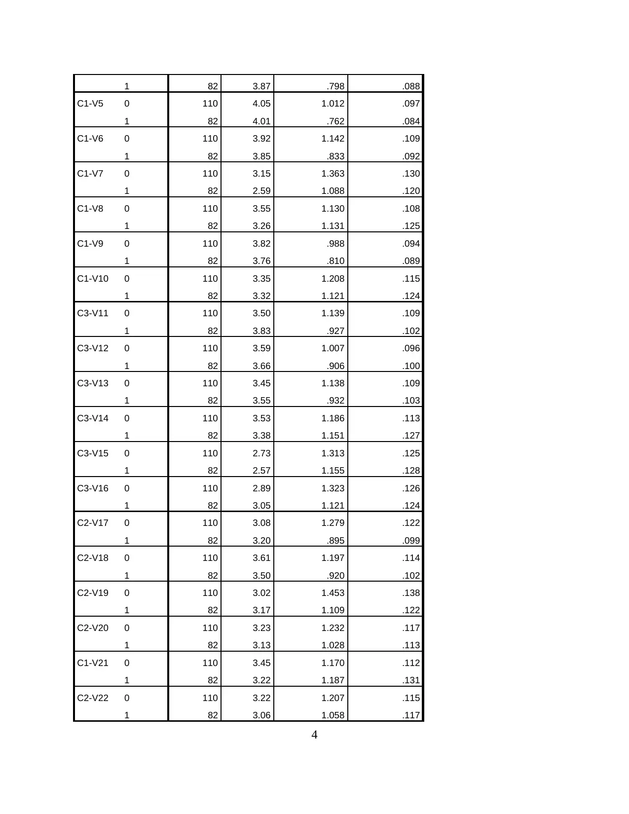
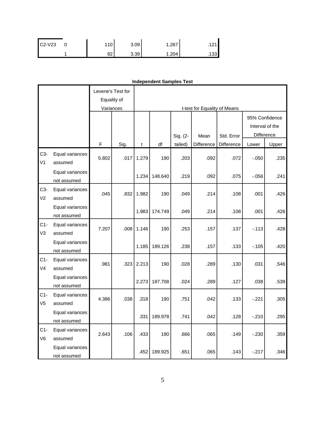
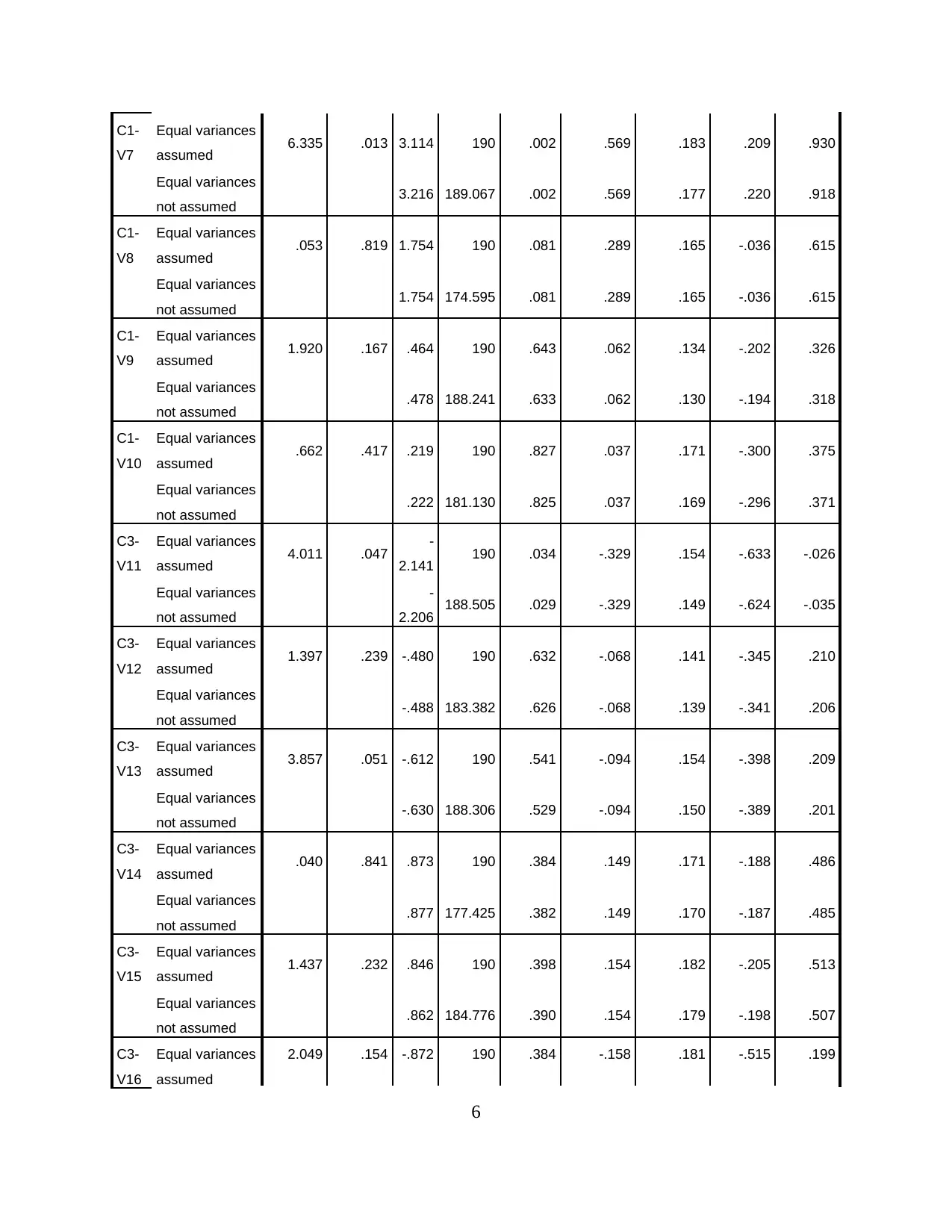
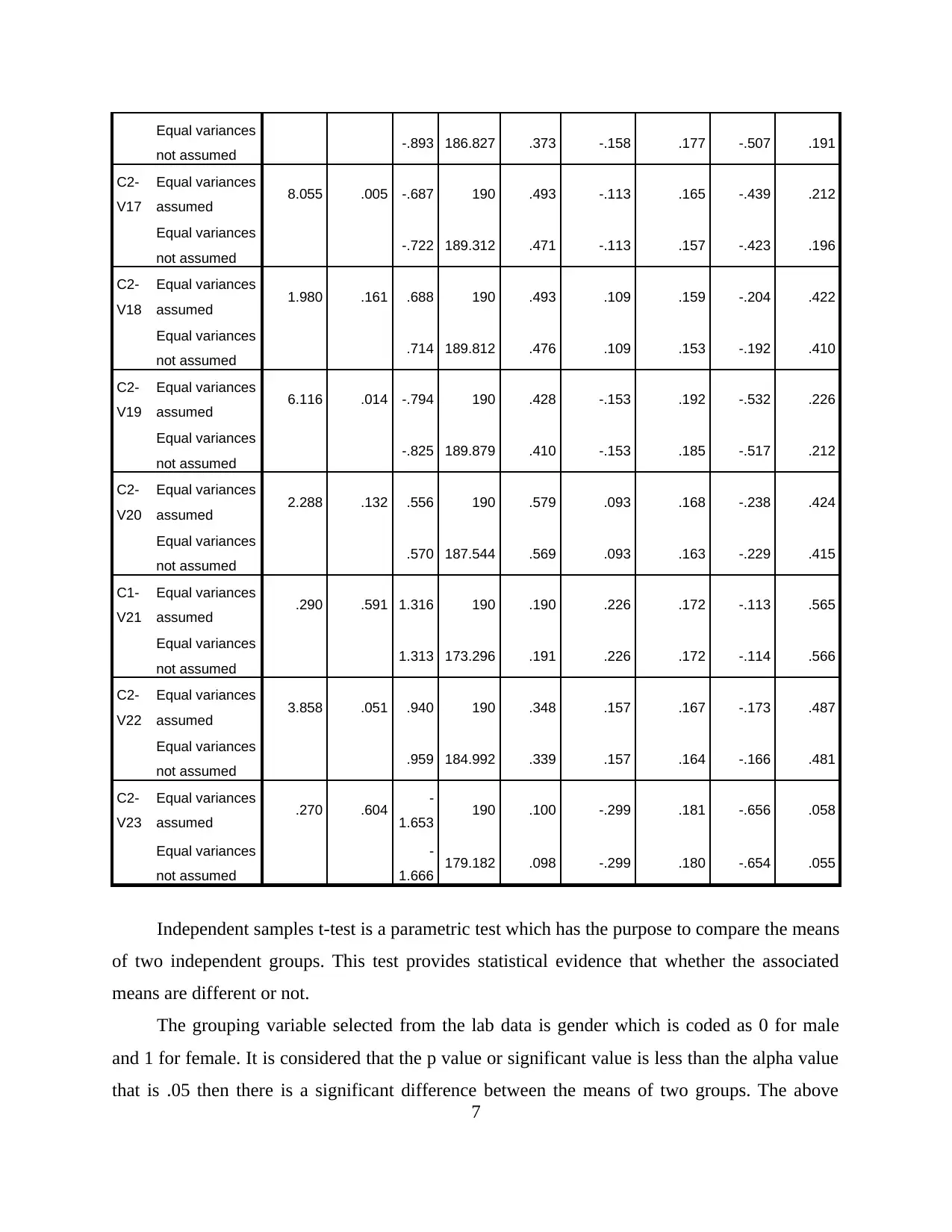
Independent samples t-test is a parametric test which has the purpose to compare the means
of two independent groups. This test provides statistical evidence that whether the associated
means are different or not.
The grouping variable selected from the lab data is gender which is coded as 0 for male
and 1 for female. It is considered that the p value or significant value is less than the alpha value
that is .05 then there is a significant difference between the means of two groups. The above
7

results shows that p value of the variables C3-V2, C1-V4, C1-V7 and C3-V11 is less than .05
which means these variables has different means for males and females.
6. Chi-square test
Gender * Position Class Crosstabulation
Count
Position Class
Total0 2 3 4 5 6
Gender 0 24 29 35 17 3 2 110
1 4 12 25 25 9 7 82
Total 28 41 60 42 12 9 192
Chi-Square Tests
Value df
Asymptotic
Significance
(2-sided)
Exact Sig. (2-
sided)
Exact Sig. (1-
sided)
Point
Probability
Pearson Chi-Square 26.789a 5 .000 .000
Likelihood Ratio 28.307 5 .000 .000
Fisher's Exact Test 27.036 .000
Linear-by-Linear
Association 25.529b 1 .000 .000 .000 .000
N of Valid Cases 192
a. 1 cells (8.3%) have expected count less than 5. The minimum expected count is 3.84.
b. The standardized statistic is 5.053.
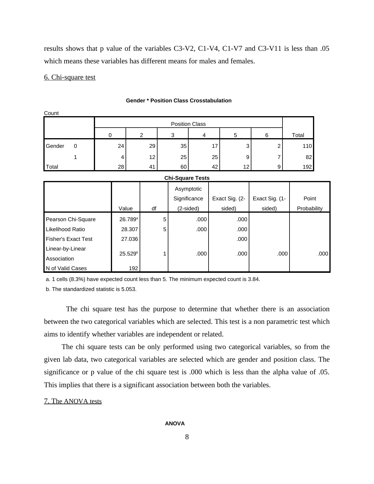
The chi square test has the purpose to determine that whether there is an association
between the two categorical variables which are selected. This test is a non parametric test which
aims to identify whether variables are independent or related.
The chi square tests can be only performed using two categorical variables, so from the
given lab data, two categorical variables are selected which are gender and position class. The
significance or p value of the chi square test is .000 which is less than the alpha value of .05.
This implies that there is a significant association between both the variables.
7. The ANOVA tests
ANOVA
8

Sum of Squares df Mean Square F Sig.
C3-V1 Between Groups 1.682 5 .336 1.378 .234
Within Groups 45.396 186 .244
Total 47.078 191
C3-V2 Between Groups 1.633 5 .327 .584 .712
Within Groups 104.070 186 .560
Total 105.703 191
C1-V3 Between Groups 1.686 5 .337 .374 .866
Within Groups 167.793 186 .902
Total 169.479 191
C1-V4 Between Groups 3.257 5 .651 .794 .555
Within Groups 152.555 186 .820
Total 155.813 191
C1-V5 Between Groups 6.598 5 1.320 1.613 .158
Within Groups 152.147 186 .818
Total 158.745 191
C1-V6 Between Groups 7.779 5 1.556 1.516 .187
Within Groups 190.924 186 1.026
Total 198.703 191
C1-V7 Between Groups 6.064 5 1.213 .734 .599
Within Groups 307.431 186 1.653
Total 313.495 191
C1-V8 Between Groups 4.152 5 .830 .636 .672
Within Groups 242.676 186 1.305
Total 246.828 191
C1-V9 Between Groups 5.511 5 1.102 1.330 .253
Within Groups 154.156 186 .829
Total 159.667 191
C1-V10 Between Groups 1.993 5 .399 .286 .920
Within Groups 259.002 186 1.392
Total 260.995 191
C3-V11 Between Groups 6.101 5 1.220 1.080 .373
Within Groups 210.102 186 1.130
Total 216.203 191
C3-V12 Between Groups .486 5 .097 .102 .992
Within Groups 176.759 186 .950
Total 177.245 191
9

C3-V13 Between Groups .937 5 .187 .165 .975
Within Groups 211.057 186 1.135
Total 211.995 191
C3-V14 Between Groups 3.089 5 .618 .444 .817
Within Groups 258.656 186 1.391
Total 261.745 191
C3-V15 Between Groups 9.195 5 1.839 1.188 .316
Within Groups 287.800 186 1.547
Total 296.995 191
C3-V16 Between Groups 8.079 5 1.616 1.052 .388
Within Groups 285.588 186 1.535
Total 293.667 191
C2-V17 Between Groups 7.705 5 1.541 1.214 .304
Within Groups 236.040 186 1.269
Total 243.745 191
C2-V18 Between Groups 3.049 5 .610 .510 .768
Within Groups 222.201 186 1.195
Total 225.250 191
C2-V19 Between Groups 6.536 5 1.307 .750 .587
Within Groups 324.131 186 1.743
Total 330.667 191
C2-V20 Between Groups 4.156 5 .831 .626 .680
Within Groups 247.094 186 1.328
Total 251.250 191
C1-V21 Between Groups 2.874 5 .575 .407 .844
Within Groups 262.746 186 1.413
Total 265.620 191
C2-V22 Between Groups 5.842 5 1.168 .888 .490
Within Groups 244.778 186 1.316
Total 250.620 191
C2-V23 Between Groups 3.733 5 .747 .474 .795
Within Groups 293.079 186 1.576
Total 296.813 191
10

One way Anova is a statistical test which is conducted for the purpose of comparing the
groups which can be two or more than two. This test provides statistical evidence that whether
the differences between the groups are significant or not.
As Anova test can check the mean differences of the variable having two or more groups,
the factor variable which has selected is employee evaluation having 5 groups. It has been
considered for ANOVA test that if the p value is less than the alpha value of .05, then there is a
statistically significant difference between the groups. The above results shows that in none of
the variables, the p value is less than .05 which means that there is no statistical difference
between the groups of employee evaluation.
8. Linear/multiple regression tests
Model Summary
Model R R Square
Adjusted R
Square
Std. Error of the
Estimate
1 .173a .030 .014 .493
a. Predictors: (Constant), Employee Evaluation, Gender, Position Class
ANOVAa
Model Sum of Squares df Mean Square F Sig.
1 Regression 1.409 3 .470 1.933 .126b
Residual 45.669 188 .243
Total 47.078 191
a. Dependent Variable: C3-V1
b. Predictors: (Constant), Employee Evaluation, Gender, Position Class
Coefficientsa
Model
Unstandardized Coefficients
Standardized
Coefficients
t Sig.B Std. Error Beta
1 (Constant) 4.669 .095 49.132 .000
Gender -.133 .077 -.133 -1.721 .087
Position Class .009 .028 .029 .333 .739
Employee Evaluation .045 .028 .134 1.593 .113
a. Dependent Variable: C3-V1
In the above regression analysis, C3-V1 is considered as dependent variable and Employee
Evaluation, Gender & Position Class is considered as independent variable. The R square of the
11

above model is .030 which means the C3-V1 is impacted to 30% from Employee Evaluation,
Gender & Position Class.
9. Factor analysis and confirmatory tests
Communalities
Initial Extraction
C3-V1 1.000 .707
C3-V2 1.000 .678
C1-V3 1.000 .680
C1-V4 1.000 .723
C1-V5 1.000 .691
C1-V6 1.000 .704
C1-V7 1.000 .617
C1-V8 1.000 .570
C1-V9 1.000 .518
C1-V10 1.000 .527
C3-V11 1.000 .731
C3-V12 1.000 .708
C3-V13 1.000 .421
C3-V14 1.000 .594
C3-V15 1.000 .583
C3-V16 1.000 .621
C2-V17 1.000 .611
C2-V18 1.000 .702
C2-V19 1.000 .562
C2-V20 1.000 .514
C1-V21 1.000 .597
C2-V22 1.000 .511
C2-V23 1.000 .520
Extraction Method: Principal
Component Analysis.
Total Variance Explained
Component
Initial Eigenvalues Extraction Sums of Squared Loadings
Total % of Variance Cumulative % Total % of Variance Cumulative %
1 6.354 27.626 27.626 6.354 27.626 27.626
12

2 2.761 12.005 39.630 2.761 12.005 39.630
3 1.576 6.852 46.482 1.576 6.852 46.482
4 1.277 5.552 52.035 1.277 5.552 52.035
5 1.120 4.870 56.905 1.120 4.870 56.905
6 1.005 4.370 61.275 1.005 4.370 61.275
7 .957 4.160 65.435
8 .835 3.629 69.064
9 .813 3.535 72.600
10 .755 3.282 75.881
11 .650 2.825 78.706
12 .611 2.655 81.361
13 .588 2.555 83.916
14 .544 2.363 86.279
15 .491 2.137 88.416
16 .479 2.083 90.499
17 .436 1.895 92.395
18 .361 1.569 93.963
19 .354 1.540 95.503
20 .322 1.402 96.905
21 .287 1.249 98.155
22 .218 .948 99.103
23 .206 .897 100.000
Extraction Method: Principal Component Analysis.
The factor analysis and confirmatory test are conducted with purpose to analyses that
whether the selected data fits to the hypothesized measurement model. The extraction value of
all the variables is more than .5 which means the data is a more than average fit to the hypothesis
model.
13