SPSS: Bivariate and Multivariate Regression Analysis Assignment
VerifiedAdded on 2023/06/05
|31
|6069
|78
Homework Assignment
AI Summary
This assignment solution provides a detailed analysis of bivariate and multivariate regression using SPSS. The first part focuses on bivariate regression, examining the relationship between stress and the number of visits to health professionals (timedrs). It includes outlier analysis, correlation analysis, and the development of a regression equation to predict timedrs based on stress levels. The second part extends the analysis to multivariate regression, incorporating physical and mental health symptoms as additional independent variables. The solution includes ANOVA tables, regression coefficients, and interpretations of R-squared values, assessing the significance and predictive power of the models. The assignment concludes with a discussion of the findings and their implications, emphasizing the importance of considering multiple factors in predicting healthcare utilization.

Statistics
Student Name:
Instructor Name:
Course Number:
20 September 2018
Student Name:
Instructor Name:
Course Number:
20 September 2018
Paraphrase This Document
Need a fresh take? Get an instant paraphrase of this document with our AI Paraphraser
SPSS Bivariate Regression Assignment
1. As with all data, it is important to take a look at the data to examine potential
univariate and bivariate outliers. Use procedures described in earlier assignments
to examine outliers and to get to know your data (if you see potential outliers you
can transform the data, delete the outliers, or leave them in the data; justify your
reasoning). For this assignment focus on only two variables: timedrs, stress.
Supply a box plot and/or histogram of the two variables.
Answer
From table 1 below, it can be seen that the average number of visits to health
professionals was 7.80 with a standard deviation of 10.95. The skewness value is
3.25 implying the variable is highly skewed.
Table 1: Statistics
Visits to health
professionals
Stressful life events
N Valid 465 465
Missing 1 1
Mean 7.90 204.22
Median 4.00 178.00
Mode 2.00 0.00
Std. Deviation 10.95 135.79
Variance 119.87 18439.66
Skewness 3.25 1.04
Std. Error of Skewness 0.11 0.11
Kurtosis 13.10 1.80
Std. Error of Kurtosis 0.23 0.23
Range 81.00 920.00
Minimum 0.00 0.00
Maximum 81.00 920.00
Percentiles 25 2.00 98.00
50 4.00 178.00
75 10.00 278.00

Histogram and Boxplot for the stressful life events
⊘ This is a preview!⊘
Do you want full access?
Subscribe today to unlock all pages.
Trusted by 1+ million students worldwide
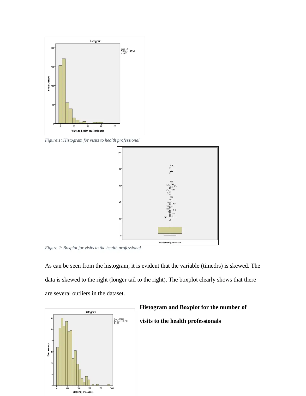
Figure 2: Boxplot for visits to the health professional
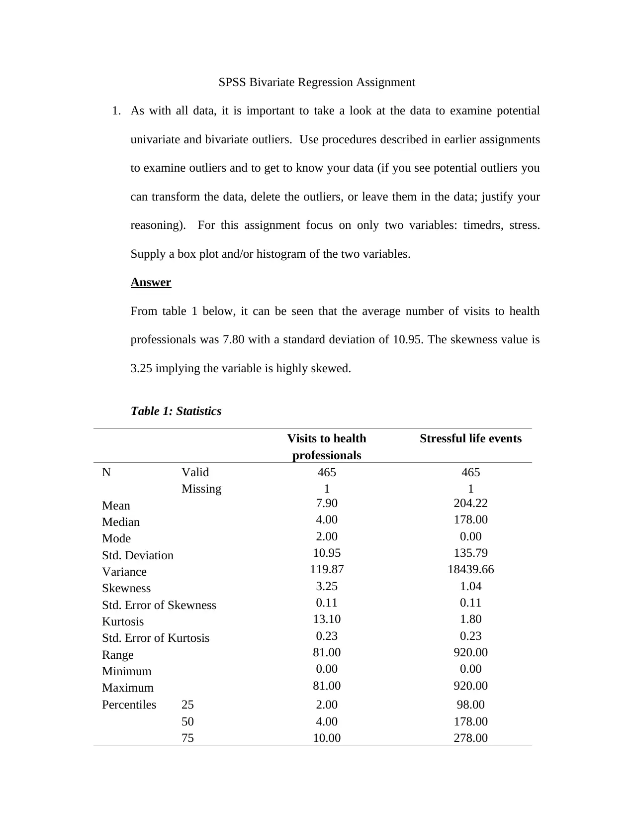
As can be seen from the histogram, it is evident that the variable (timedrs) is skewed. The
data is skewed to the right (longer tail to the right). The boxplot clearly shows that there
are several outliers in the dataset.
Histogram and Boxplot for the number of
visits to the health professionals
Figure 1: Histogram for visits to health professional
Paraphrase This Document
Need a fresh take? Get an instant paraphrase of this document with our AI Paraphraser
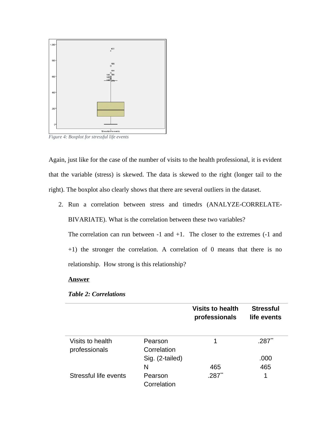
Figure 4: Boxplot for stressful life events
Again, just like for the case of the number of visits to the health professional, it is evident
that the variable (stress) is skewed. The data is skewed to the right (longer tail to the
right). The boxplot also clearly shows that there are several outliers in the dataset.
2. Run a correlation between stress and timedrs (ANALYZE-CORRELATE-
BIVARIATE). What is the correlation between these two variables?
The correlation can run between -1 and +1. The closer to the extremes (-1 and
+1) the stronger the correlation. A correlation of 0 means that there is no
relationship. How strong is this relationship?
Answer
Table 2: Correlations
Visits to health
professionals
Stressful
life events
Visits to health
professionals
Pearson
Correlation
1 .287**
Sig. (2-tailed) .000
N 465 465
Stressful life events Pearson
Correlation
.287** 1
Sig. (2-tailed) .000
N 465 465
**. Correlation is significant at the 0.01 level (2-tailed).
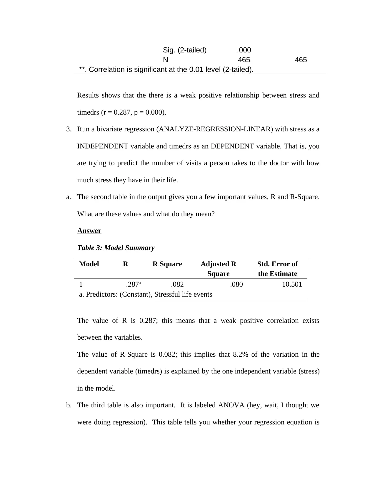
Results shows that the there is a weak positive relationship between stress and
timedrs (r = 0.287, p = 0.000).
3. Run a bivariate regression (ANALYZE-REGRESSION-LINEAR) with stress as a
INDEPENDENT variable and timedrs as an DEPENDENT variable. That is, you
are trying to predict the number of visits a person takes to the doctor with how
much stress they have in their life.
a. The second table in the output gives you a few important values, R and R-Square.
What are these values and what do they mean?
Answer
Table 3: Model Summary
Model R R Square Adjusted R
Square
Std. Error of
the Estimate
1 .287a .082 .080 10.501
a. Predictors: (Constant), Stressful life events
The value of R is 0.287; this means that a weak positive correlation exists
between the variables.
The value of R-Square is 0.082; this implies that 8.2% of the variation in the
dependent variable (timedrs) is explained by the one independent variable (stress)
in the model.
b. The third table is also important. It is labeled ANOVA (hey, wait, I thought we
were doing regression). This table tells you whether your regression equation is
N 465 465
**. Correlation is significant at the 0.01 level (2-tailed).
Results shows that the there is a weak positive relationship between stress and
timedrs (r = 0.287, p = 0.000).
3. Run a bivariate regression (ANALYZE-REGRESSION-LINEAR) with stress as a
INDEPENDENT variable and timedrs as an DEPENDENT variable. That is, you
are trying to predict the number of visits a person takes to the doctor with how
much stress they have in their life.
a. The second table in the output gives you a few important values, R and R-Square.
What are these values and what do they mean?
Answer
Table 3: Model Summary
Model R R Square Adjusted R
Square
Std. Error of
the Estimate
1 .287a .082 .080 10.501
a. Predictors: (Constant), Stressful life events
The value of R is 0.287; this means that a weak positive correlation exists
between the variables.
The value of R-Square is 0.082; this implies that 8.2% of the variation in the
dependent variable (timedrs) is explained by the one independent variable (stress)
in the model.
b. The third table is also important. It is labeled ANOVA (hey, wait, I thought we
were doing regression). This table tells you whether your regression equation is
⊘ This is a preview!⊘
Do you want full access?
Subscribe today to unlock all pages.
Trusted by 1+ million students worldwide
significant (thus does the regression line significantly predict the DV). Is your
regression line significant?
Answer
Table 4: ANOVA
Model Sum of
Squares
df Mean
Square
F Sig.
1 Regressi
on
4568.402 1 4568.402 41.432 .000b
Residual 51051.047 463 110.261
Total 55619.449 464
a. Dependent Variable: Visits to health professionals
b. Predictors: (Constant), Stressful life events
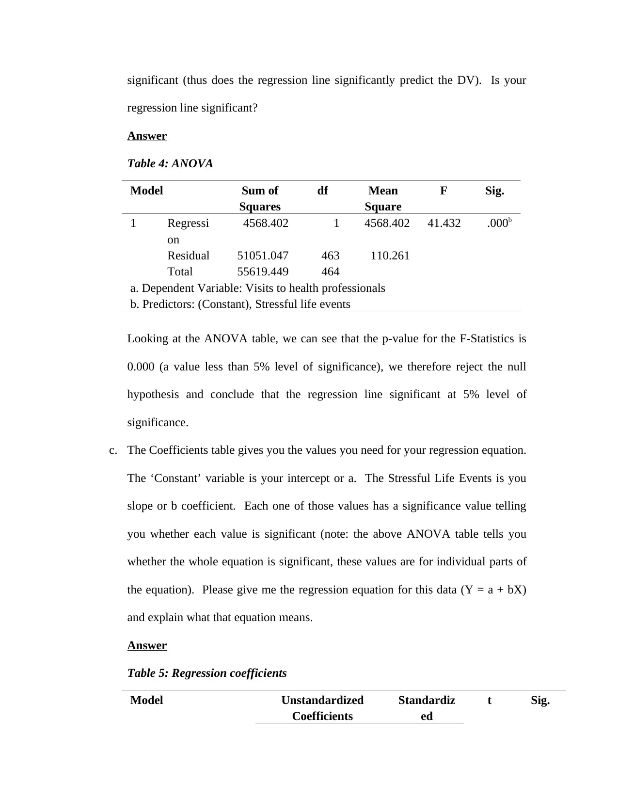
Looking at the ANOVA table, we can see that the p-value for the F-Statistics is
0.000 (a value less than 5% level of significance), we therefore reject the null
hypothesis and conclude that the regression line significant at 5% level of
significance.
c. The Coefficients table gives you the values you need for your regression equation.
The ‘Constant’ variable is your intercept or a. The Stressful Life Events is you
slope or b coefficient. Each one of those values has a significance value telling
you whether each value is significant (note: the above ANOVA table tells you
whether the whole equation is significant, these values are for individual parts of
the equation). Please give me the regression equation for this data (Y = a + bX)
and explain what that equation means.
Answer
Table 5: Regression coefficients
Model Unstandardized
Coefficients
Standardiz
ed
t Sig.
regression line significant?
Answer
Table 4: ANOVA
Model Sum of
Squares
df Mean
Square
F Sig.
1 Regressi
on
4568.402 1 4568.402 41.432 .000b
Residual 51051.047 463 110.261
Total 55619.449 464
a. Dependent Variable: Visits to health professionals
b. Predictors: (Constant), Stressful life events
Looking at the ANOVA table, we can see that the p-value for the F-Statistics is
0.000 (a value less than 5% level of significance), we therefore reject the null
hypothesis and conclude that the regression line significant at 5% level of
significance.
c. The Coefficients table gives you the values you need for your regression equation.
The ‘Constant’ variable is your intercept or a. The Stressful Life Events is you
slope or b coefficient. Each one of those values has a significance value telling
you whether each value is significant (note: the above ANOVA table tells you
whether the whole equation is significant, these values are for individual parts of
the equation). Please give me the regression equation for this data (Y = a + bX)
and explain what that equation means.
Answer
Table 5: Regression coefficients
Model Unstandardized
Coefficients
Standardiz
ed
t Sig.
Paraphrase This Document
Need a fresh take? Get an instant paraphrase of this document with our AI Paraphraser
Coefficient
s
B Std. Error Beta
1 (Constant) 3.182 .880 3.616 .000
Stressful life
events
.023 .004 .287 6.437 .000
a. Dependent Variable: Visits to health professionals
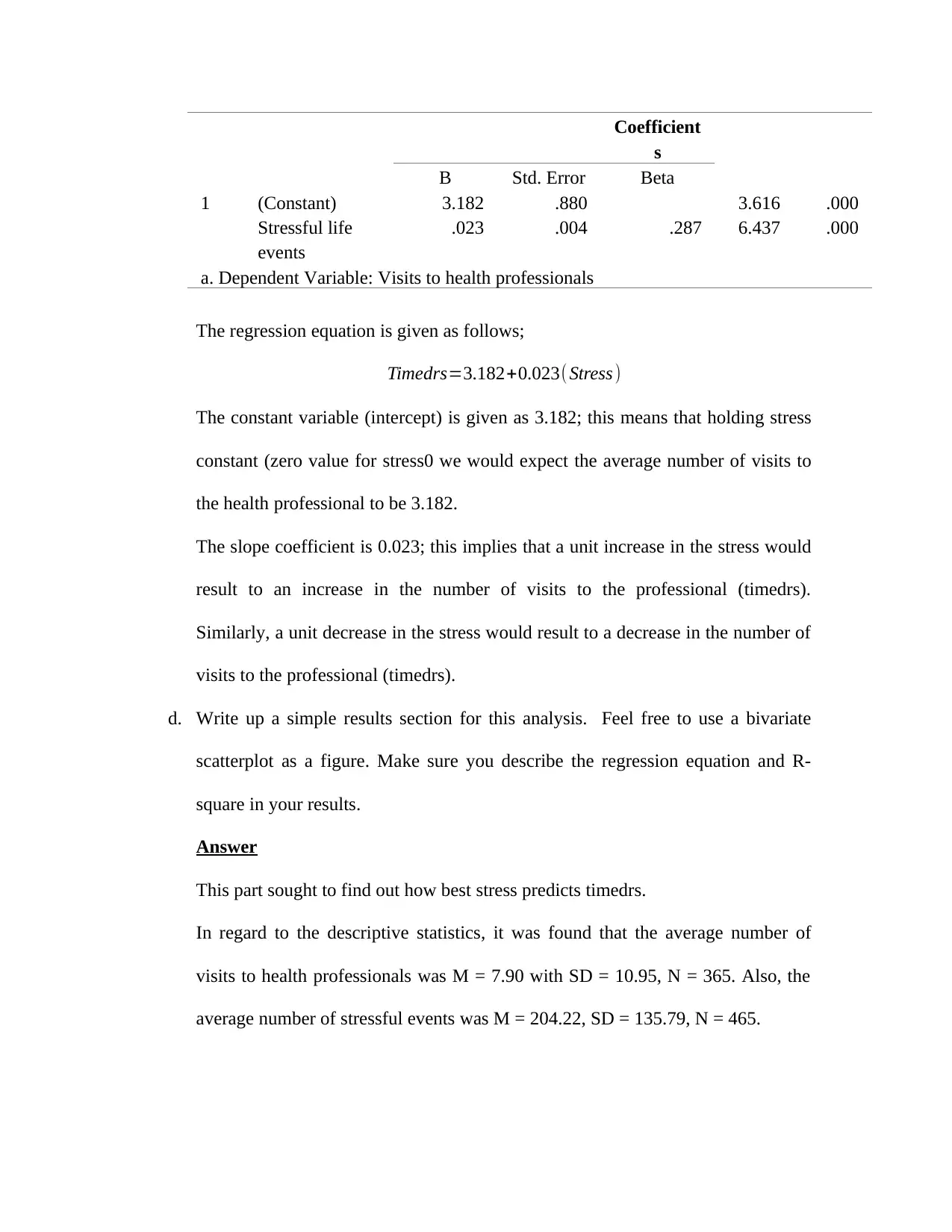
The regression equation is given as follows;
Timedrs=3.182+0.023( Stress)
The constant variable (intercept) is given as 3.182; this means that holding stress
constant (zero value for stress0 we would expect the average number of visits to
the health professional to be 3.182.
The slope coefficient is 0.023; this implies that a unit increase in the stress would
result to an increase in the number of visits to the professional (timedrs).
Similarly, a unit decrease in the stress would result to a decrease in the number of
visits to the professional (timedrs).
d. Write up a simple results section for this analysis. Feel free to use a bivariate
scatterplot as a figure. Make sure you describe the regression equation and R-
square in your results.
Answer
This part sought to find out how best stress predicts timedrs.
In regard to the descriptive statistics, it was found that the average number of
visits to health professionals was M = 7.90 with SD = 10.95, N = 365. Also, the
average number of stressful events was M = 204.22, SD = 135.79, N = 465.
s
B Std. Error Beta
1 (Constant) 3.182 .880 3.616 .000
Stressful life
events
.023 .004 .287 6.437 .000
a. Dependent Variable: Visits to health professionals
The regression equation is given as follows;
Timedrs=3.182+0.023( Stress)
The constant variable (intercept) is given as 3.182; this means that holding stress
constant (zero value for stress0 we would expect the average number of visits to
the health professional to be 3.182.
The slope coefficient is 0.023; this implies that a unit increase in the stress would
result to an increase in the number of visits to the professional (timedrs).
Similarly, a unit decrease in the stress would result to a decrease in the number of
visits to the professional (timedrs).
d. Write up a simple results section for this analysis. Feel free to use a bivariate
scatterplot as a figure. Make sure you describe the regression equation and R-
square in your results.
Answer
This part sought to find out how best stress predicts timedrs.
In regard to the descriptive statistics, it was found that the average number of
visits to health professionals was M = 7.90 with SD = 10.95, N = 365. Also, the
average number of stressful events was M = 204.22, SD = 135.79, N = 465.
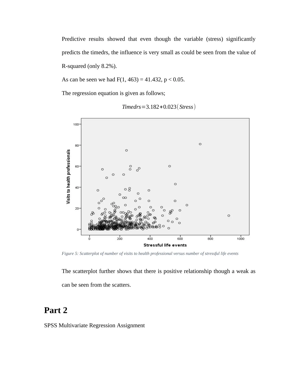
Predictive results showed that even though the variable (stress) significantly
predicts the timedrs, the influence is very small as could be seen from the value of
R-squared (only 8.2%).
As can be seen we had F(1, 463) = 41.432, p < 0.05.
The regression equation is given as follows;
Timedrs=3.182+0.023( Stress)
Figure 5: Scatterplot of number of visits to health professional versus number of stressful life events
The scatterplot further shows that there is positive relationship though a weak as
can be seen from the scatters.
Part 2
SPSS Multivariate Regression Assignment
⊘ This is a preview!⊘
Do you want full access?
Subscribe today to unlock all pages.
Trusted by 1+ million students worldwide
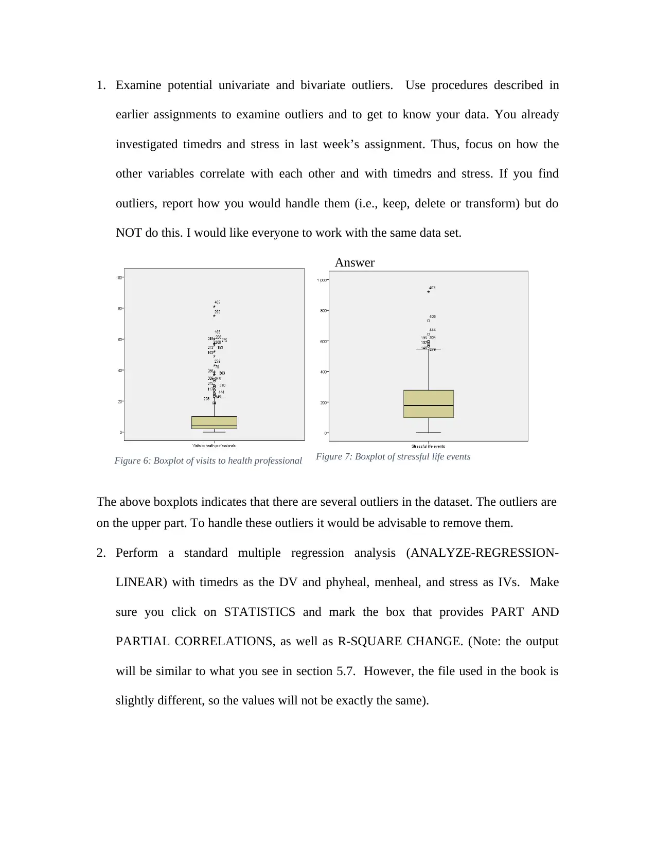
1. Examine potential univariate and bivariate outliers. Use procedures described in
earlier assignments to examine outliers and to get to know your data. You already
investigated timedrs and stress in last week’s assignment. Thus, focus on how the
other variables correlate with each other and with timedrs and stress. If you find
outliers, report how you would handle them (i.e., keep, delete or transform) but do
NOT do this. I would like everyone to work with the same data set.
Answer
Figure 7: Boxplot of stressful life events
The above boxplots indicates that there are several outliers in the dataset. The outliers are
on the upper part. To handle these outliers it would be advisable to remove them.
2. Perform a standard multiple regression analysis (ANALYZE-REGRESSION-
LINEAR) with timedrs as the DV and phyheal, menheal, and stress as IVs. Make
sure you click on STATISTICS and mark the box that provides PART AND
PARTIAL CORRELATIONS, as well as R-SQUARE CHANGE. (Note: the output
will be similar to what you see in section 5.7. However, the file used in the book is
slightly different, so the values will not be exactly the same).
Figure 6: Boxplot of visits to health professional
Paraphrase This Document
Need a fresh take? Get an instant paraphrase of this document with our AI Paraphraser
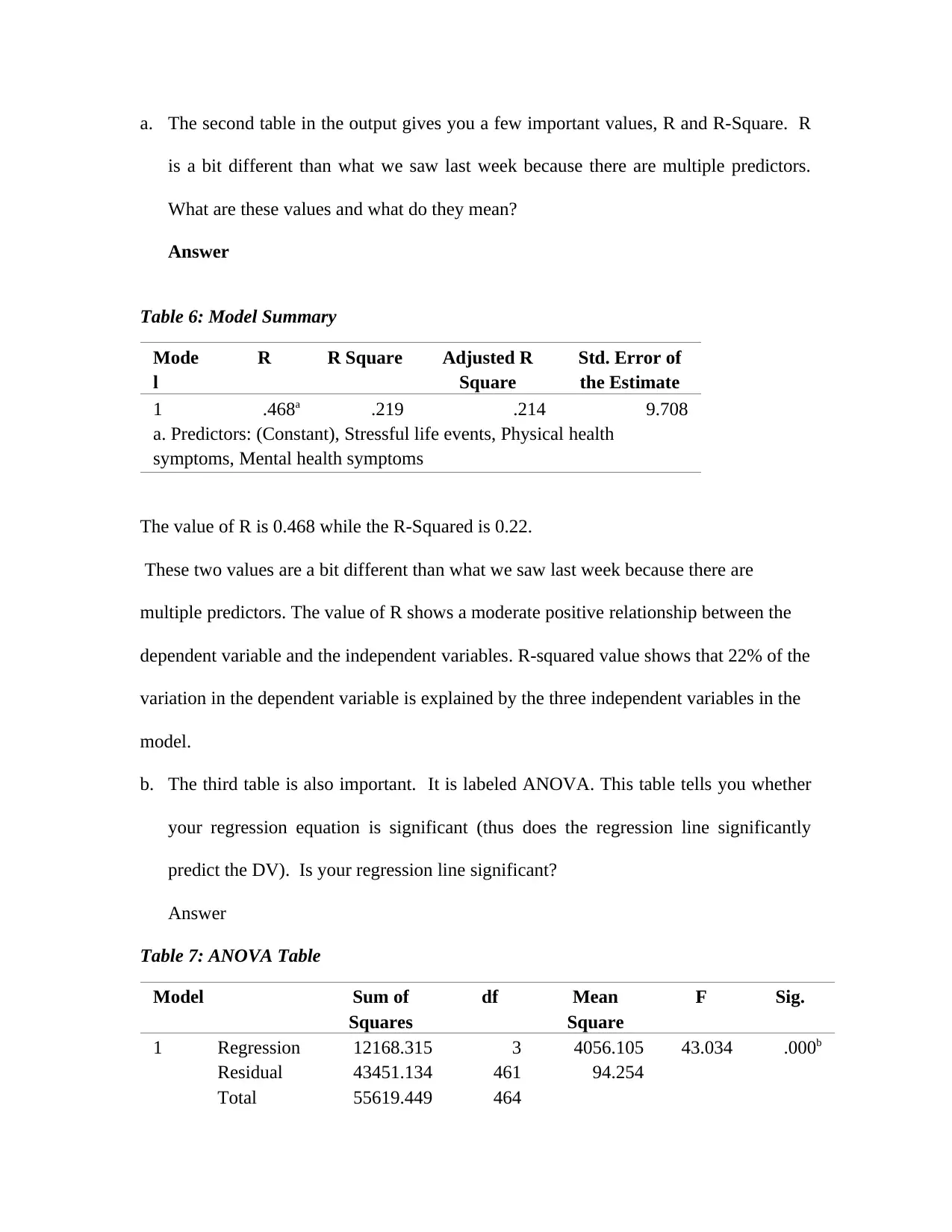
a. The second table in the output gives you a few important values, R and R-Square. R
is a bit different than what we saw last week because there are multiple predictors.
What are these values and what do they mean?
Answer
Table 6: Model Summary
Mode
l
R R Square Adjusted R
Square
Std. Error of
the Estimate
1 .468a .219 .214 9.708
a. Predictors: (Constant), Stressful life events, Physical health
symptoms, Mental health symptoms
The value of R is 0.468 while the R-Squared is 0.22.
These two values are a bit different than what we saw last week because there are
multiple predictors. The value of R shows a moderate positive relationship between the
dependent variable and the independent variables. R-squared value shows that 22% of the
variation in the dependent variable is explained by the three independent variables in the
model.
b. The third table is also important. It is labeled ANOVA. This table tells you whether
your regression equation is significant (thus does the regression line significantly
predict the DV). Is your regression line significant?
Answer
Table 7: ANOVA Table
Model Sum of
Squares
df Mean
Square
F Sig.
1 Regression 12168.315 3 4056.105 43.034 .000b
Residual 43451.134 461 94.254
Total 55619.449 464
a. Dependent Variable: Visits to health professionals
b. Predictors: (Constant), Stressful life events, Physical health symptoms, Mental health
symptoms
Looking at the ANOVA table, we can see that the p-value for the F-Statistics is p<.001 (a
value less than 5% level of significance), we therefore reject the null hypothesis and
conclude that the regression line significant at 5% level of significance [F(3, 461) =
43.03, p < 0.05].
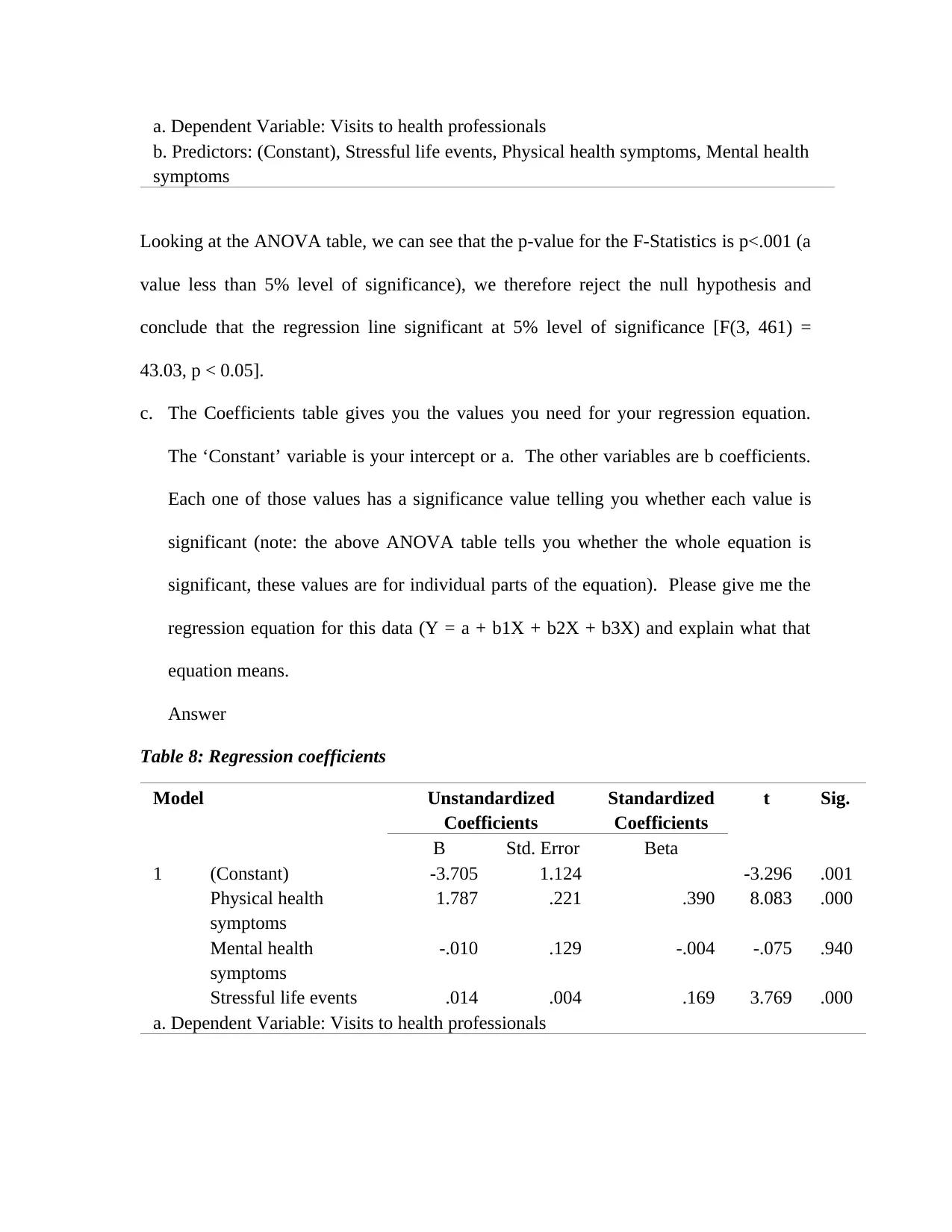
c. The Coefficients table gives you the values you need for your regression equation.
The ‘Constant’ variable is your intercept or a. The other variables are b coefficients.
Each one of those values has a significance value telling you whether each value is
significant (note: the above ANOVA table tells you whether the whole equation is
significant, these values are for individual parts of the equation). Please give me the
regression equation for this data (Y = a + b1X + b2X + b3X) and explain what that
equation means.
Answer
Table 8: Regression coefficients
Model Unstandardized
Coefficients
Standardized
Coefficients
t Sig.
B Std. Error Beta
1 (Constant) -3.705 1.124 -3.296 .001
Physical health
symptoms
1.787 .221 .390 8.083 .000
Mental health
symptoms
-.010 .129 -.004 -.075 .940
Stressful life events .014 .004 .169 3.769 .000
a. Dependent Variable: Visits to health professionals
b. Predictors: (Constant), Stressful life events, Physical health symptoms, Mental health
symptoms
Looking at the ANOVA table, we can see that the p-value for the F-Statistics is p<.001 (a
value less than 5% level of significance), we therefore reject the null hypothesis and
conclude that the regression line significant at 5% level of significance [F(3, 461) =
43.03, p < 0.05].
c. The Coefficients table gives you the values you need for your regression equation.
The ‘Constant’ variable is your intercept or a. The other variables are b coefficients.
Each one of those values has a significance value telling you whether each value is
significant (note: the above ANOVA table tells you whether the whole equation is
significant, these values are for individual parts of the equation). Please give me the
regression equation for this data (Y = a + b1X + b2X + b3X) and explain what that
equation means.
Answer
Table 8: Regression coefficients
Model Unstandardized
Coefficients
Standardized
Coefficients
t Sig.
B Std. Error Beta
1 (Constant) -3.705 1.124 -3.296 .001
Physical health
symptoms
1.787 .221 .390 8.083 .000
Mental health
symptoms
-.010 .129 -.004 -.075 .940
Stressful life events .014 .004 .169 3.769 .000
a. Dependent Variable: Visits to health professionals
⊘ This is a preview!⊘
Do you want full access?
Subscribe today to unlock all pages.
Trusted by 1+ million students worldwide
1 out of 31
Your All-in-One AI-Powered Toolkit for Academic Success.
+13062052269
info@desklib.com
Available 24*7 on WhatsApp / Email
![[object Object]](/_next/static/media/star-bottom.7253800d.svg)
Unlock your academic potential
Copyright © 2020–2026 A2Z Services. All Rights Reserved. Developed and managed by ZUCOL.