SPSS Statistics Assignment

This SPSS Statistics Assignment analyzes the difference between practice test scores of low-income students participating in an afterschool program and state averages. It also examines if students have improved their test scores in reading, math, and science, and if gender differences exist in these scores.

SPSS Statistics Assignment
Student Name:
Instructor Name:
Course Number:
10 April 2019

Question 1: Is there a significant difference between the practice test scores of low income
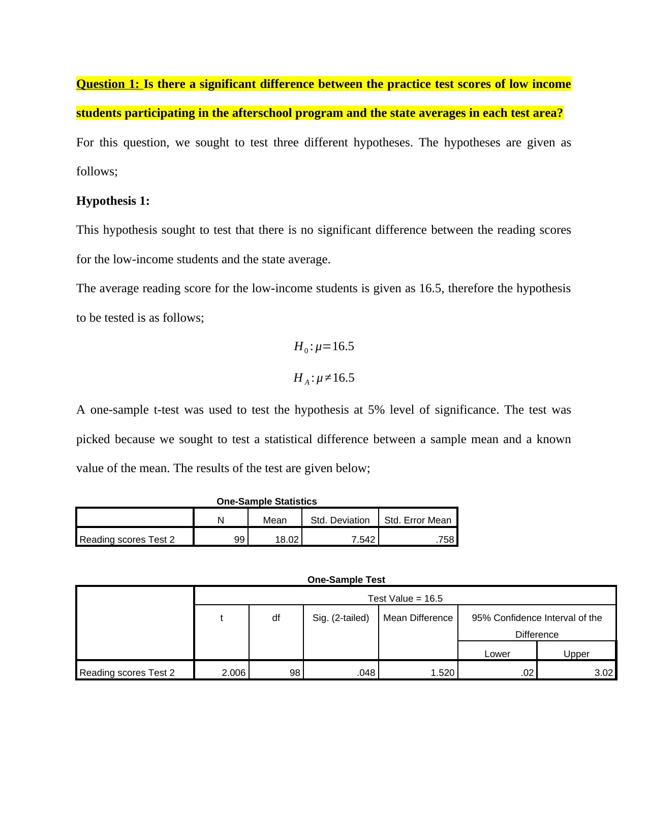
students participating in the afterschool program and the state averages in each test area?
For this question, we sought to test three different hypotheses. The hypotheses are given as
follows;
Hypothesis 1:
This hypothesis sought to test that there is no significant difference between the reading scores
for the low-income students and the state average.
The average reading score for the low-income students is given as 16.5, therefore the hypothesis
to be tested is as follows;
H0 : μ=16.5
H A : μ ≠16.5
A one-sample t-test was used to test the hypothesis at 5% level of significance. The test was
picked because we sought to test a statistical difference between a sample mean and a known
value of the mean. The results of the test are given below;
One-Sample Statistics
N Mean Std. Deviation Std. Error Mean
Reading scores Test 2 99 18.02 7.542 .758
One-Sample Test
Test Value = 16.5
t df Sig. (2-tailed) Mean Difference 95% Confidence Interval of the
Difference
Lower Upper
Reading scores Test 2 2.006 98 .048 1.520 .02 3.02

The state average for the reading scores was averagely higher (M = 18.02, SD = 7.54) as
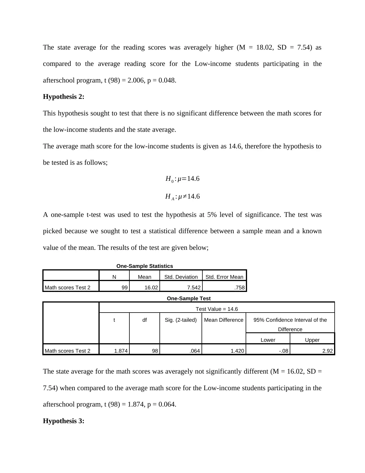
compared to the average reading score for the Low-income students participating in the
afterschool program, t (98) = 2.006, p = 0.048.
Hypothesis 2:
This hypothesis sought to test that there is no significant difference between the math scores for
the low-income students and the state average.
The average math score for the low-income students is given as 14.6, therefore the hypothesis to
be tested is as follows;
H0 : μ=14.6
H A : μ ≠14.6
A one-sample t-test was used to test the hypothesis at 5% level of significance. The test was
picked because we sought to test a statistical difference between a sample mean and a known
value of the mean. The results of the test are given below;
One-Sample Statistics
N Mean Std. Deviation Std. Error Mean
Math scores Test 2 99 16.02 7.542 .758
One-Sample Test
Test Value = 14.6
t df Sig. (2-tailed) Mean Difference 95% Confidence Interval of the
Difference
Lower Upper
Math scores Test 2 1.874 98 .064 1.420 -.08 2.92
The state average for the math scores was averagely not significantly different (M = 16.02, SD =
7.54) when compared to the average math score for the Low-income students participating in the
afterschool program, t (98) = 1.874, p = 0.064.
Hypothesis 3:

This hypothesis sought to test that there is no significant difference between the science scores
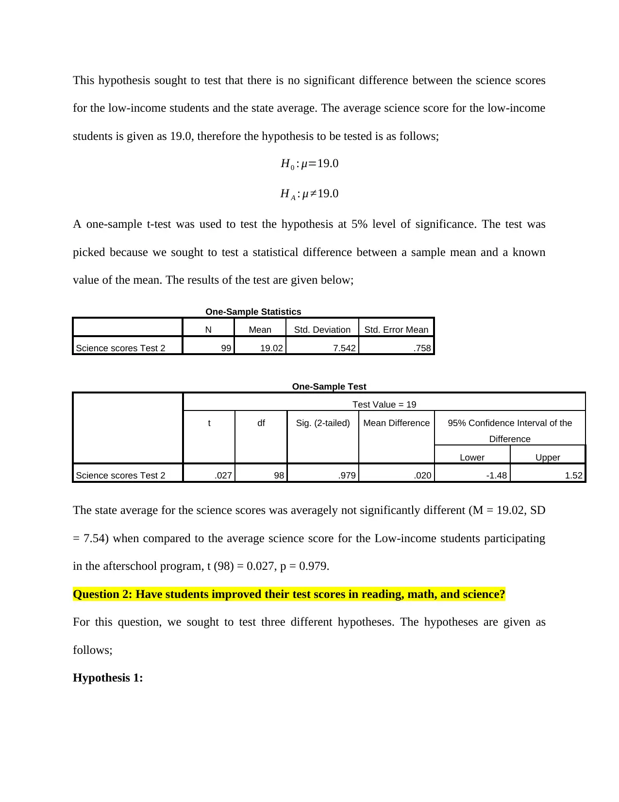
for the low-income students and the state average. The average science score for the low-income
students is given as 19.0, therefore the hypothesis to be tested is as follows;
H0 : μ=19.0
H A : μ ≠19.0
A one-sample t-test was used to test the hypothesis at 5% level of significance. The test was
picked because we sought to test a statistical difference between a sample mean and a known
value of the mean. The results of the test are given below;
One-Sample Statistics
N Mean Std. Deviation Std. Error Mean
Science scores Test 2 99 19.02 7.542 .758
One-Sample Test
Test Value = 19
t df Sig. (2-tailed) Mean Difference 95% Confidence Interval of the
Difference
Lower Upper
Science scores Test 2 .027 98 .979 .020 -1.48 1.52
The state average for the science scores was averagely not significantly different (M = 19.02, SD
= 7.54) when compared to the average science score for the Low-income students participating
in the afterschool program, t (98) = 0.027, p = 0.979.
Question 2: Have students improved their test scores in reading, math, and science?
For this question, we sought to test three different hypotheses. The hypotheses are given as
follows;
Hypothesis 1:

This hypothesis sought to test that there is no significant difference between the reading scores
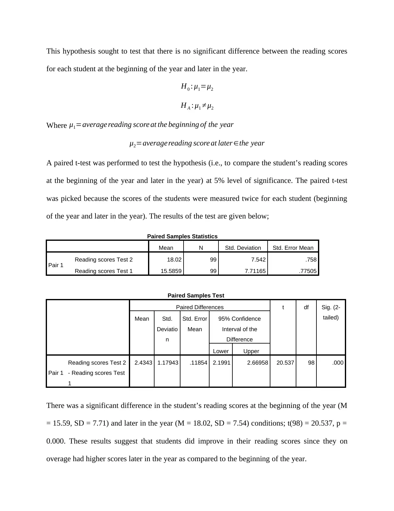
for each student at the beginning of the year and later in the year.
H0 : μ1=μ2
H A : μ1 ≠ μ2
Where μ1=average reading score at the beginning of the year
μ2=averagereading score at later ∈the year
A paired t-test was performed to test the hypothesis (i.e., to compare the student’s reading scores
at the beginning of the year and later in the year) at 5% level of significance. The paired t-test
was picked because the scores of the students were measured twice for each student (beginning
of the year and later in the year). The results of the test are given below;
Paired Samples Statistics
Mean N Std. Deviation Std. Error Mean
Pair 1 Reading scores Test 2 18.02 99 7.542 .758
Reading scores Test 1 15.5859 99 7.71165 .77505
Paired Samples Test
Paired Differences t df Sig. (2-
tailed)Mean Std.
Deviatio
n
Std. Error
Mean
95% Confidence
Interval of the
Difference
Lower Upper
Pair 1
Reading scores Test 2
- Reading scores Test
1
2.4343 1.17943 .11854 2.1991 2.66958 20.537 98 .000
There was a significant difference in the student’s reading scores at the beginning of the year (M
= 15.59, SD = 7.71) and later in the year (M = 18.02, SD = 7.54) conditions; t(98) = 20.537, p =
0.000. These results suggest that students did improve in their reading scores since they on
overage had higher scores later in the year as compared to the beginning of the year.

Hypothesis 2:
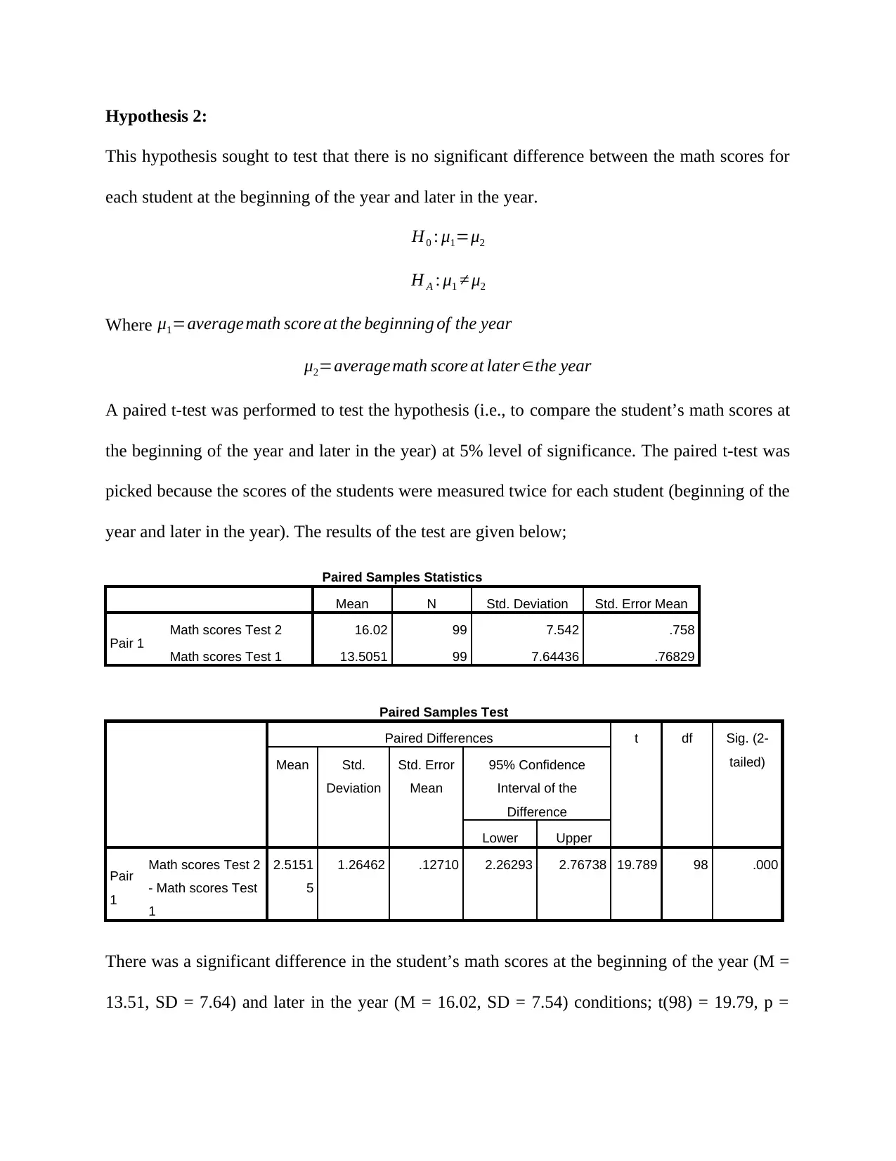
This hypothesis sought to test that there is no significant difference between the math scores for
each student at the beginning of the year and later in the year.
H0 : μ1=μ2
H A : μ1 ≠ μ2
Where μ1=average math score at the beginning of the year
μ2=average math score at later ∈the year
A paired t-test was performed to test the hypothesis (i.e., to compare the student’s math scores at
the beginning of the year and later in the year) at 5% level of significance. The paired t-test was
picked because the scores of the students were measured twice for each student (beginning of the
year and later in the year). The results of the test are given below;
Paired Samples Statistics
Mean N Std. Deviation Std. Error Mean
Pair 1 Math scores Test 2 16.02 99 7.542 .758
Math scores Test 1 13.5051 99 7.64436 .76829
Paired Samples Test
Paired Differences t df Sig. (2-
tailed)Mean Std.
Deviation
Std. Error
Mean
95% Confidence
Interval of the
Difference
Lower Upper
Pair
1
Math scores Test 2
- Math scores Test
1
2.5151
5
1.26462 .12710 2.26293 2.76738 19.789 98 .000
There was a significant difference in the student’s math scores at the beginning of the year (M =
13.51, SD = 7.64) and later in the year (M = 16.02, SD = 7.54) conditions; t(98) = 19.79, p =

0.000. These results suggest that students did improve in their math scores since they on overage
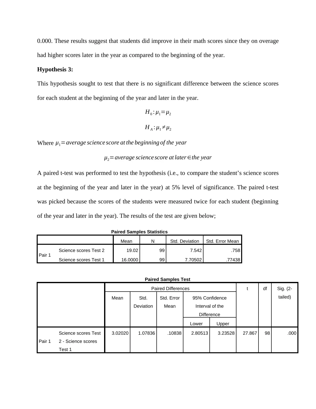
had higher scores later in the year as compared to the beginning of the year.
Hypothesis 3:
This hypothesis sought to test that there is no significant difference between the science scores
for each student at the beginning of the year and later in the year.
H0 : μ1=μ2
H A : μ1 ≠ μ2
Where μ1=average science score at the beginning of the year
μ2=average science score at later ∈the year
A paired t-test was performed to test the hypothesis (i.e., to compare the student’s science scores
at the beginning of the year and later in the year) at 5% level of significance. The paired t-test
was picked because the scores of the students were measured twice for each student (beginning
of the year and later in the year). The results of the test are given below;
Paired Samples Statistics
Mean N Std. Deviation Std. Error Mean
Pair 1 Science scores Test 2 19.02 99 7.542 .758
Science scores Test 1 16.0000 99 7.70502 .77438
Paired Samples Test
Paired Differences t df Sig. (2-
tailed)Mean Std.
Deviation
Std. Error
Mean
95% Confidence
Interval of the
Difference
Lower Upper
Pair 1
Science scores Test
2 - Science scores
Test 1
3.02020 1.07836 .10838 2.80513 3.23528 27.867 98 .000

There was a significant difference in the student’s science scores at the beginning of the year (M
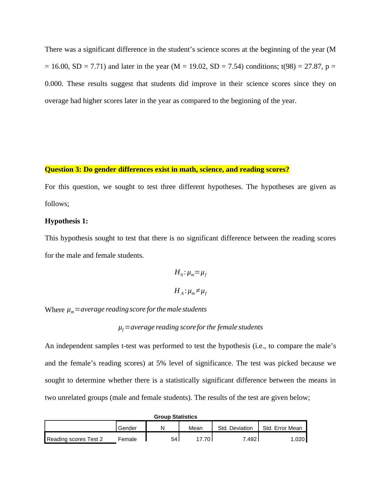
= 16.00, SD = 7.71) and later in the year (M = 19.02, SD = 7.54) conditions; t(98) = 27.87, p =
0.000. These results suggest that students did improve in their science scores since they on
overage had higher scores later in the year as compared to the beginning of the year.
Question 3: Do gender differences exist in math, science, and reading scores?
For this question, we sought to test three different hypotheses. The hypotheses are given as
follows;
Hypothesis 1:
This hypothesis sought to test that there is no significant difference between the reading scores
for the male and female students.
H0 : μm=μf
H A : μm ≠ μf
Where μm =average reading score for the male students
μf =average reading score for the female students
An independent samples t-test was performed to test the hypothesis (i.e., to compare the male’s
and the female’s reading scores) at 5% level of significance. The test was picked because we
sought to determine whether there is a statistically significant difference between the means in
two unrelated groups (male and female students). The results of the test are given below;
Group Statistics
Gender N Mean Std. Deviation Std. Error Mean
Reading scores Test 2 Female 54 17.70 7.492 1.020

Male 45 18.40 7.668 1.143
Independent Samples Test
Levene's Test for
Equality of
Variances
t-test for Equality of Means
F Sig. t df Sig. (2-
tailed)
Mean
Differen
ce
Std.
Error
Differen
ce
95% Confidence
Interval of the
Difference
Lower Upper
Reading scores
Test 2
Equal variances
assumed
.027 .871 -.456 97 .650 -.696 1.528 -3.730 2.337
Equal variances
not assumed
-.455 92.998 .650 -.696 1.532 -3.738 2.345
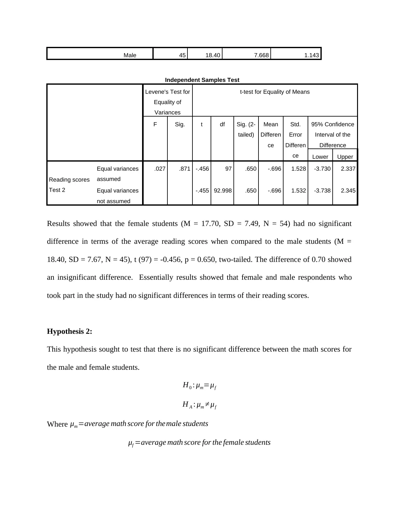
Results showed that the female students (M = 17.70, SD = 7.49, N = 54) had no significant
difference in terms of the average reading scores when compared to the male students (M =
18.40, SD = 7.67, N = 45), t (97) = -0.456, p = 0.650, two-tailed. The difference of 0.70 showed
an insignificant difference. Essentially results showed that female and male respondents who
took part in the study had no significant differences in terms of their reading scores.
Hypothesis 2:
This hypothesis sought to test that there is no significant difference between the math scores for
the male and female students.
H0 : μm=μf
H A : μm ≠ μf
Where μm =average math score for themale students
μf =average math score for the female students

An independent samples t-test was performed to test the hypothesis (i.e., to compare the male’s
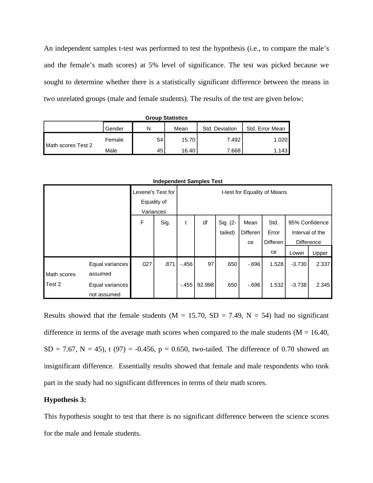
and the female’s math scores) at 5% level of significance. The test was picked because we
sought to determine whether there is a statistically significant difference between the means in
two unrelated groups (male and female students). The results of the test are given below;
Group Statistics
Gender N Mean Std. Deviation Std. Error Mean
Math scores Test 2 Female 54 15.70 7.492 1.020
Male 45 16.40 7.668 1.143
Independent Samples Test
Levene's Test for
Equality of
Variances
t-test for Equality of Means
F Sig. t df Sig. (2-
tailed)
Mean
Differen
ce
Std.
Error
Differen
ce
95% Confidence
Interval of the
Difference
Lower Upper
Math scores
Test 2
Equal variances
assumed
.027 .871 -.456 97 .650 -.696 1.528 -3.730 2.337
Equal variances
not assumed
-.455 92.998 .650 -.696 1.532 -3.738 2.345
Results showed that the female students (M = 15.70, SD = 7.49, N = 54) had no significant
difference in terms of the average math scores when compared to the male students (M = 16.40,
SD = 7.67, N = 45), t (97) = -0.456, p = 0.650, two-tailed. The difference of 0.70 showed an
insignificant difference. Essentially results showed that female and male respondents who took
part in the study had no significant differences in terms of their math scores.
Hypothesis 3:
This hypothesis sought to test that there is no significant difference between the science scores
for the male and female students.

H0 : μm=μf
H A : μm ≠ μf
Where μm =average science score for the male students
μf =average science score for the female students
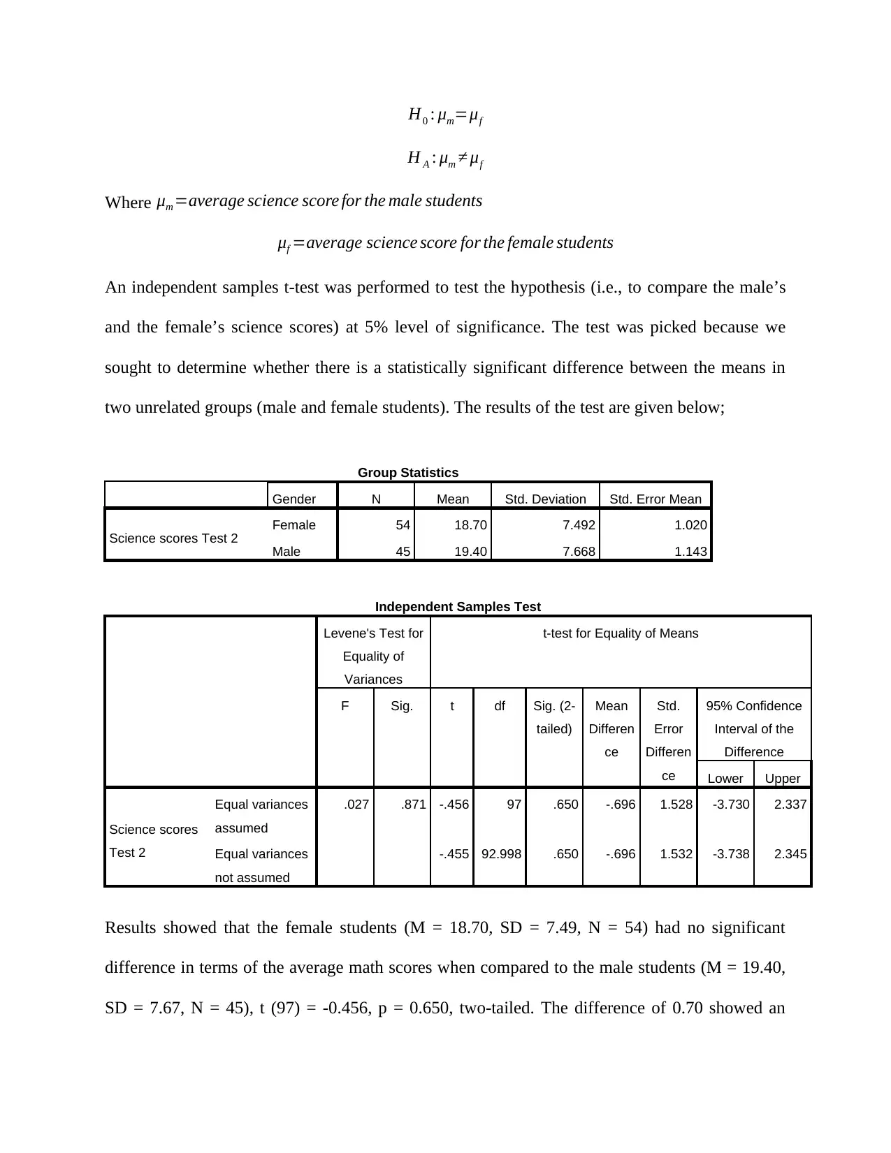
An independent samples t-test was performed to test the hypothesis (i.e., to compare the male’s
and the female’s science scores) at 5% level of significance. The test was picked because we
sought to determine whether there is a statistically significant difference between the means in
two unrelated groups (male and female students). The results of the test are given below;
Group Statistics
Gender N Mean Std. Deviation Std. Error Mean
Science scores Test 2 Female 54 18.70 7.492 1.020
Male 45 19.40 7.668 1.143
Independent Samples Test
Levene's Test for
Equality of
Variances
t-test for Equality of Means
F Sig. t df Sig. (2-
tailed)
Mean
Differen
ce
Std.
Error
Differen
ce
95% Confidence
Interval of the
Difference
Lower Upper
Science scores
Test 2
Equal variances
assumed
.027 .871 -.456 97 .650 -.696 1.528 -3.730 2.337
Equal variances
not assumed
-.455 92.998 .650 -.696 1.532 -3.738 2.345
Results showed that the female students (M = 18.70, SD = 7.49, N = 54) had no significant
difference in terms of the average math scores when compared to the male students (M = 19.40,
SD = 7.67, N = 45), t (97) = -0.456, p = 0.650, two-tailed. The difference of 0.70 showed an

insignificant difference. Essentially results showed that female and male respondents who took
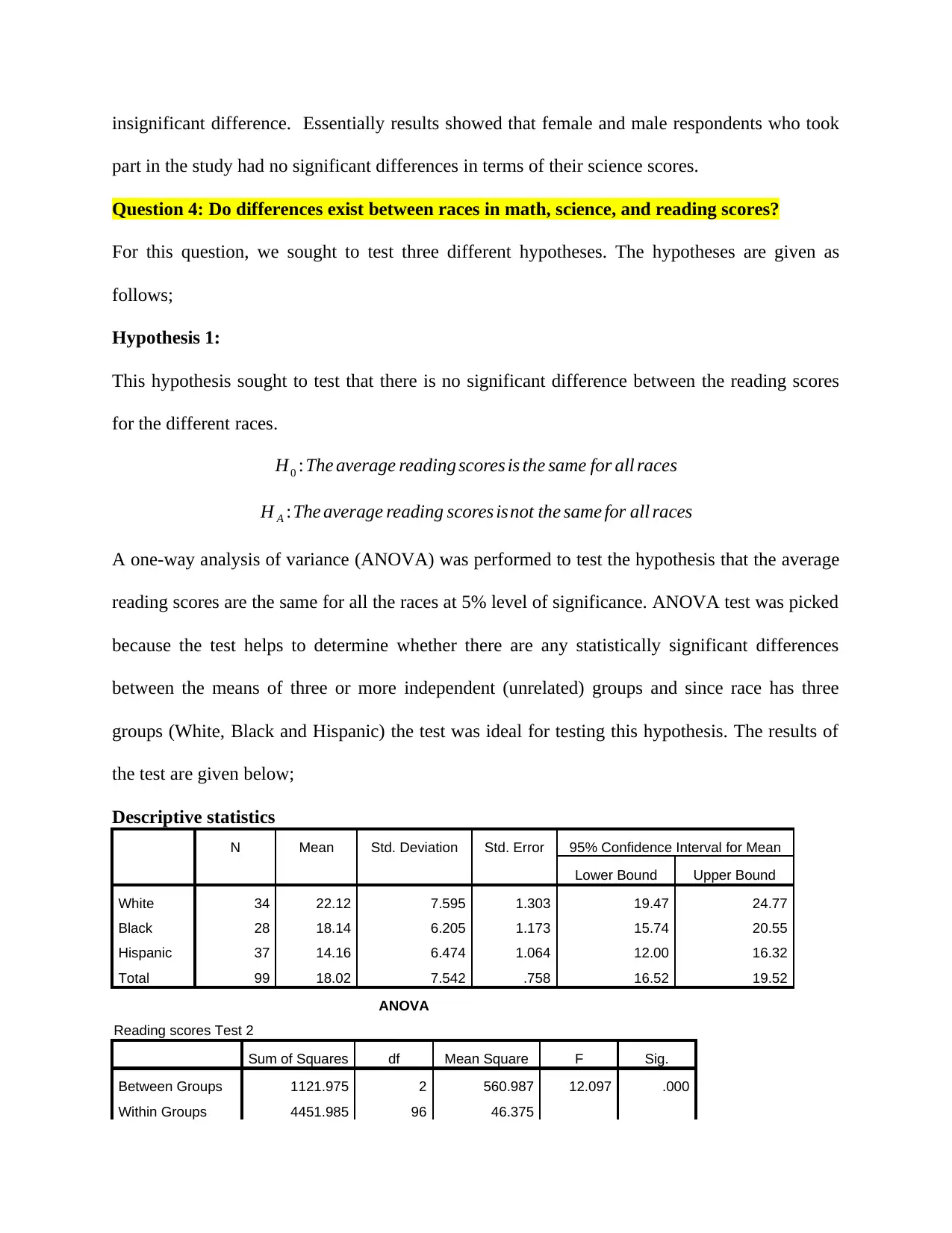
part in the study had no significant differences in terms of their science scores.
Question 4: Do differences exist between races in math, science, and reading scores?
For this question, we sought to test three different hypotheses. The hypotheses are given as
follows;
Hypothesis 1:
This hypothesis sought to test that there is no significant difference between the reading scores
for the different races.
H0 :The average reading scores is the same for all races
H A :The average reading scores isnot the same for all races
A one-way analysis of variance (ANOVA) was performed to test the hypothesis that the average
reading scores are the same for all the races at 5% level of significance. ANOVA test was picked
because the test helps to determine whether there are any statistically significant differences
between the means of three or more independent (unrelated) groups and since race has three
groups (White, Black and Hispanic) the test was ideal for testing this hypothesis. The results of
the test are given below;
Descriptive statistics
N Mean Std. Deviation Std. Error 95% Confidence Interval for Mean
Lower Bound Upper Bound
White 34 22.12 7.595 1.303 19.47 24.77
Black 28 18.14 6.205 1.173 15.74 20.55
Hispanic 37 14.16 6.474 1.064 12.00 16.32
Total 99 18.02 7.542 .758 16.52 19.52
ANOVA
Reading scores Test 2
Sum of Squares df Mean Square F Sig.
Between Groups 1121.975 2 560.987 12.097 .000
Within Groups 4451.985 96 46.375

Total 5573.960 98
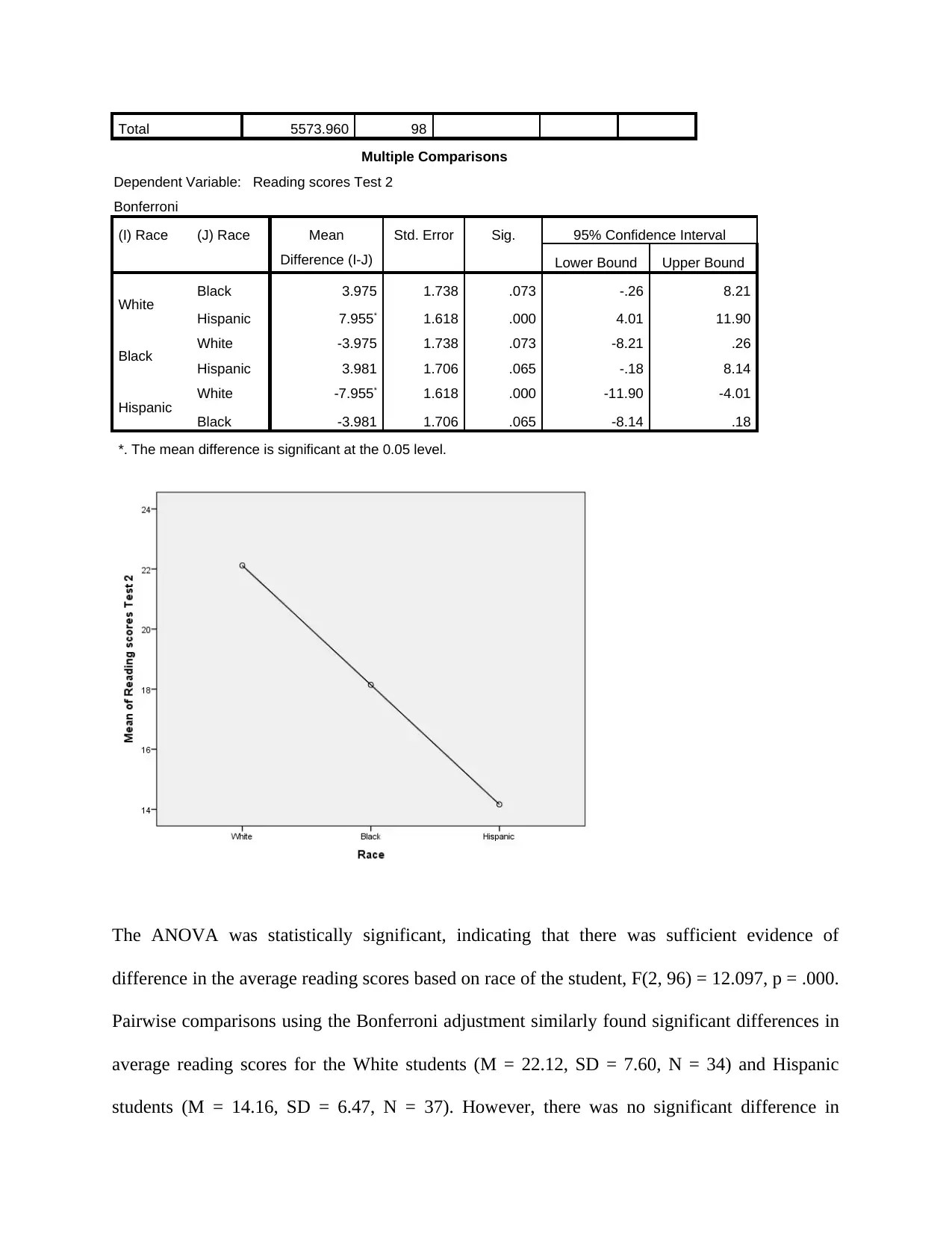
Multiple Comparisons
Dependent Variable: Reading scores Test 2
Bonferroni
(I) Race (J) Race Mean
Difference (I-J)
Std. Error Sig. 95% Confidence Interval
Lower Bound Upper Bound
White Black 3.975 1.738 .073 -.26 8.21
Hispanic 7.955* 1.618 .000 4.01 11.90
Black White -3.975 1.738 .073 -8.21 .26
Hispanic 3.981 1.706 .065 -.18 8.14
Hispanic White -7.955* 1.618 .000 -11.90 -4.01
Black -3.981 1.706 .065 -8.14 .18
*. The mean difference is significant at the 0.05 level.
The ANOVA was statistically significant, indicating that there was sufficient evidence of
difference in the average reading scores based on race of the student, F(2, 96) = 12.097, p = .000.
Pairwise comparisons using the Bonferroni adjustment similarly found significant differences in
average reading scores for the White students (M = 22.12, SD = 7.60, N = 34) and Hispanic
students (M = 14.16, SD = 6.47, N = 37). However, there was no significant difference in

average reading scores for the White students (M = 22.12, SD = 7.60, N = 34) and Black
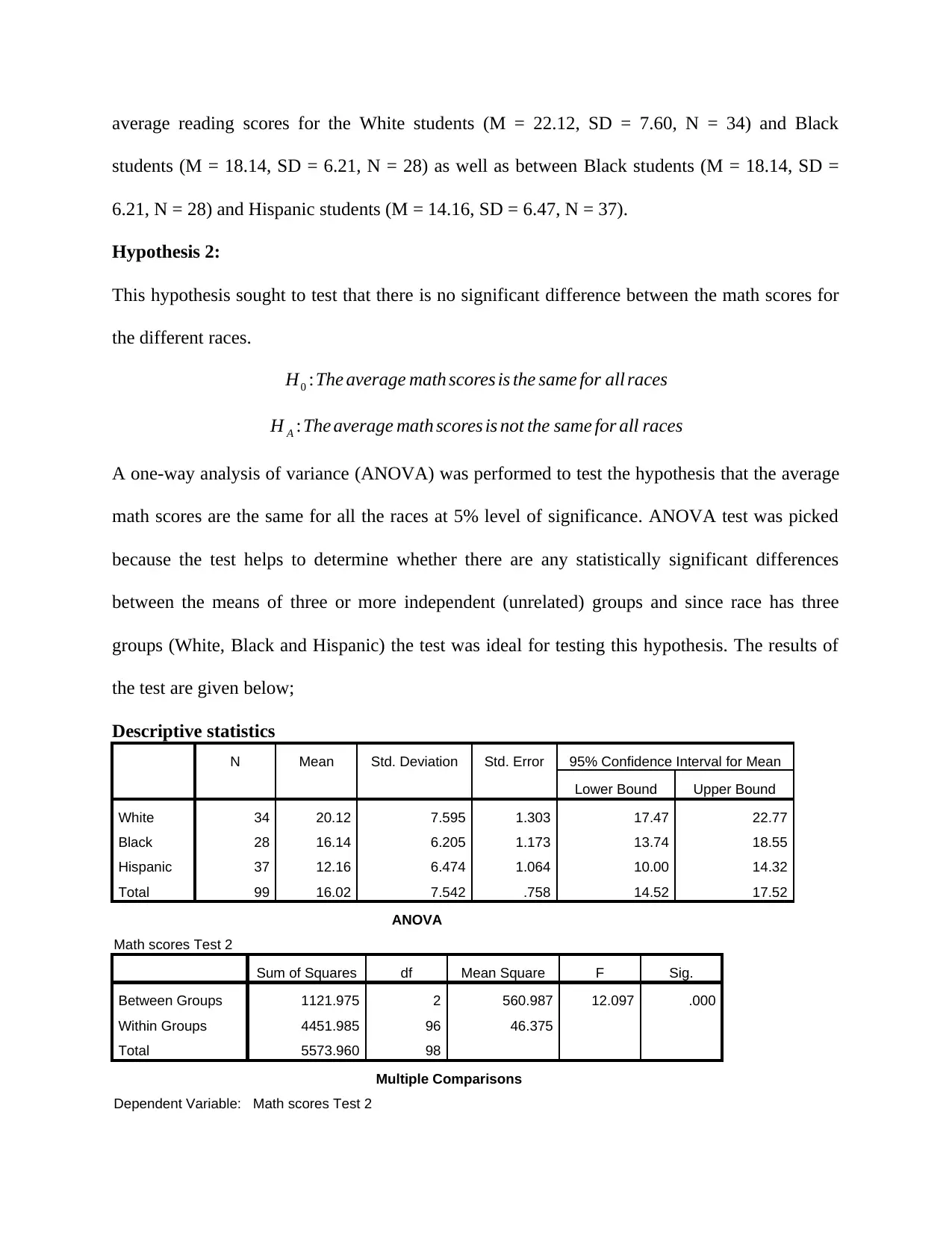
students (M = 18.14, SD = 6.21, N = 28) as well as between Black students (M = 18.14, SD =
6.21, N = 28) and Hispanic students (M = 14.16, SD = 6.47, N = 37).
Hypothesis 2:
This hypothesis sought to test that there is no significant difference between the math scores for
the different races.
H0 :The average math scores is the same for all races
H A :The average math scores is not the same for all races
A one-way analysis of variance (ANOVA) was performed to test the hypothesis that the average
math scores are the same for all the races at 5% level of significance. ANOVA test was picked
because the test helps to determine whether there are any statistically significant differences
between the means of three or more independent (unrelated) groups and since race has three
groups (White, Black and Hispanic) the test was ideal for testing this hypothesis. The results of
the test are given below;
Descriptive statistics
N Mean Std. Deviation Std. Error 95% Confidence Interval for Mean
Lower Bound Upper Bound
White 34 20.12 7.595 1.303 17.47 22.77
Black 28 16.14 6.205 1.173 13.74 18.55
Hispanic 37 12.16 6.474 1.064 10.00 14.32
Total 99 16.02 7.542 .758 14.52 17.52
ANOVA
Math scores Test 2
Sum of Squares df Mean Square F Sig.
Between Groups 1121.975 2 560.987 12.097 .000
Within Groups 4451.985 96 46.375
Total 5573.960 98
Multiple Comparisons
Dependent Variable: Math scores Test 2

Bonferroni
(I) Race (J) Race Mean Difference
(I-J)
Std. Error Sig. 95% Confidence Interval
Lower Bound Upper Bound
White Black 3.975 1.738 .073 -.26 8.21
Hispanic 7.955* 1.618 .000 4.01 11.90
Black White -3.975 1.738 .073 -8.21 .26
Hispanic 3.981 1.706 .065 -.18 8.14
Hispanic White -7.955* 1.618 .000 -11.90 -4.01
Black -3.981 1.706 .065 -8.14 .18
*. The mean difference is significant at the 0.05 level.
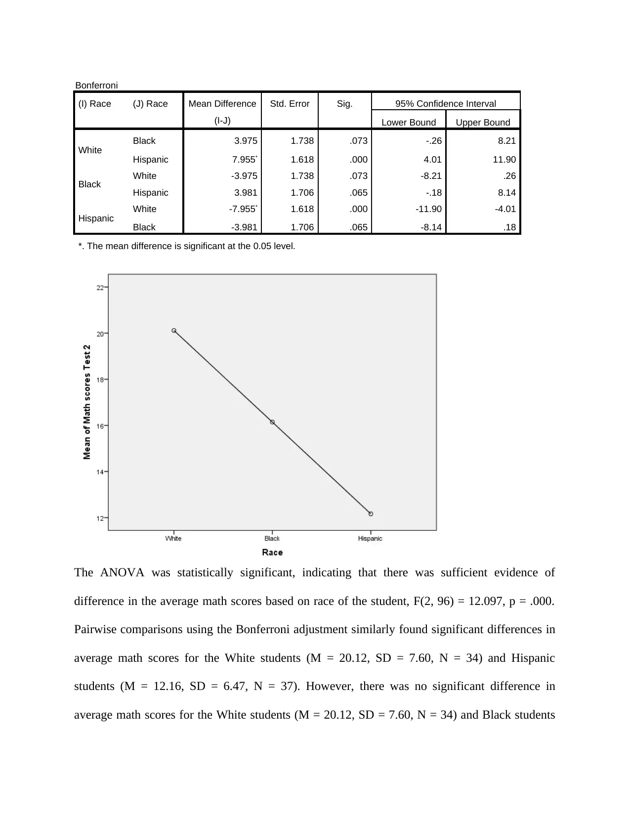
The ANOVA was statistically significant, indicating that there was sufficient evidence of
difference in the average math scores based on race of the student, F(2, 96) = 12.097, p = .000.
Pairwise comparisons using the Bonferroni adjustment similarly found significant differences in
average math scores for the White students (M = 20.12, SD = 7.60, N = 34) and Hispanic
students (M = 12.16, SD = 6.47, N = 37). However, there was no significant difference in
average math scores for the White students (M = 20.12, SD = 7.60, N = 34) and Black students

(M = 16.14, SD = 6.21, N = 28) as well as between Black students (M = 16.14, SD = 6.21, N =
28) and Hispanic students (M = 12.16, SD = 6.47, N = 37).
Hypothesis 3:
This hypothesis sought to test that there is no significant difference between the science scores
for the different races.
H0 :The average science scores isthe same for all races
H A :The average science scores is not the same for all races
A one-way analysis of variance (ANOVA) was performed to test the hypothesis that the average
science scores are the same for all the races at 5% level of significance. ANOVA test was picked
because the test helps to determine whether there are any statistically significant differences
between the means of three or more independent (unrelated) groups and since race has three
groups (White, Black and Hispanic) the test was ideal for testing this hypothesis. The results of
the test are given below;
Descriptive statistics
N Mean Std. Deviation Std. Error 95% Confidence Interval for Mean
Lower Bound Upper Bound
White 34 23.12 7.595 1.303 20.47 25.77
Black 28 19.14 6.205 1.173 16.74 21.55
Hispanic 37 15.16 6.474 1.064 13.00 17.32
Total 99 19.02 7.542 .758 17.52 20.52
ANOVA
Science scores Test 2
Sum of Squares df Mean Square F Sig.
Between Groups 1121.975 2 560.987 12.097 .000
Within Groups 4451.985 96 46.375
Total 5573.960 98
Multiple Comparisons

Dependent Variable: Science scores Test 2
Bonferroni
(I) Race (J) Race Mean Difference
(I-J)
Std. Error Sig. 95% Confidence Interval
Lower Bound Upper Bound
White Black 3.975 1.738 .073 -.26 8.21
Hispanic 7.955* 1.618 .000 4.01 11.90
Black White -3.975 1.738 .073 -8.21 .26
Hispanic 3.981 1.706 .065 -.18 8.14
Hispanic White -7.955* 1.618 .000 -11.90 -4.01
Black -3.981 1.706 .065 -8.14 .18
*. The mean difference is significant at the 0.05 level.
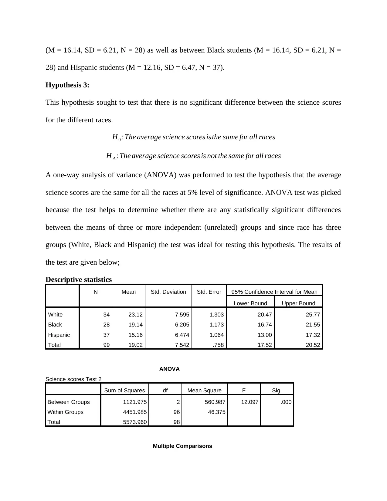
The ANOVA was statistically significant, indicating that there was sufficient evidence of
difference in the average science scores based on race of the student, F(2, 96) = 12.097, p = .000.
Pairwise comparisons using the Bonferroni adjustment similarly found significant differences in
average science scores for the White students (M = 23.12, SD = 7.60, N = 34) and Hispanic
students (M = 15.16, SD = 6.47, N = 37). However, there was no significant difference in
average science scores for the White students (M = 23.12, SD = 7.60, N = 34) and Black students

(M = 19.14, SD = 6.21, N = 28) as well as between Black students (M = 19.14, SD = 6.21, N =
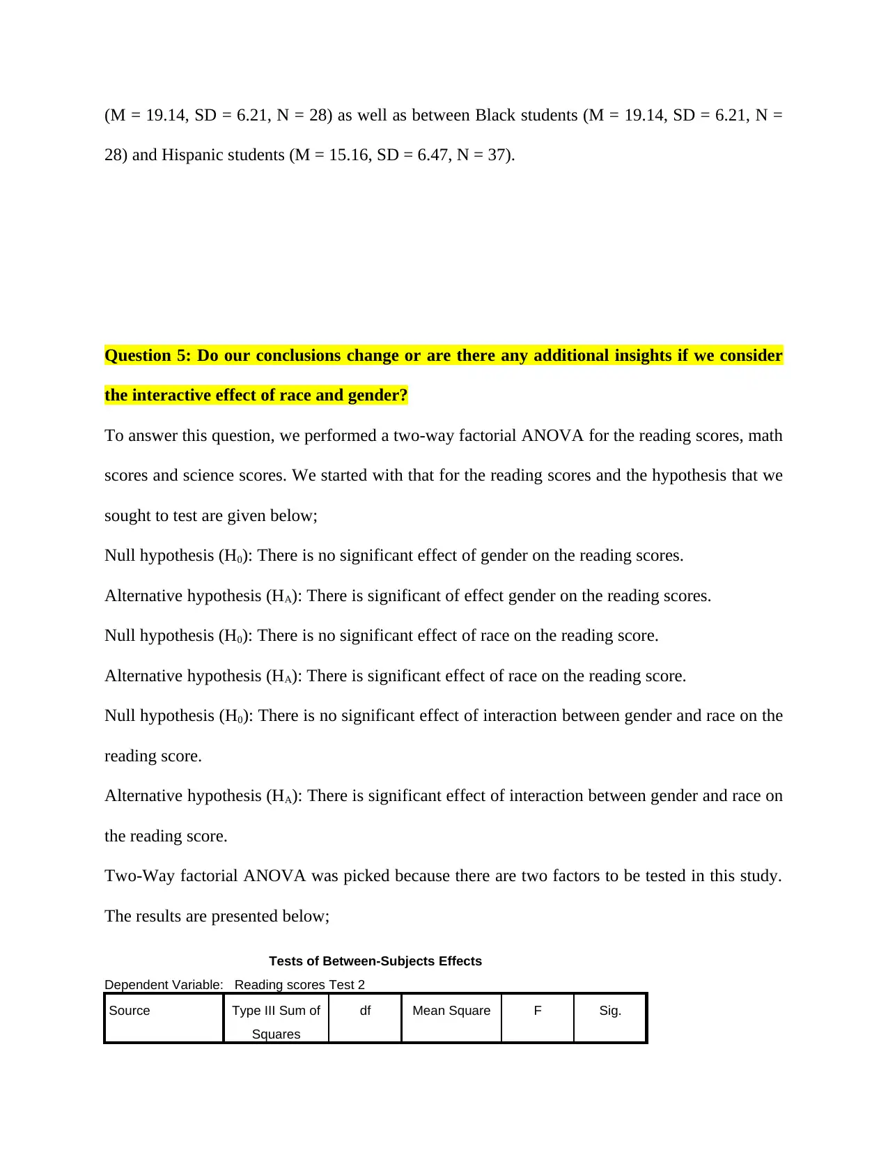
28) and Hispanic students (M = 15.16, SD = 6.47, N = 37).
Question 5: Do our conclusions change or are there any additional insights if we consider
the interactive effect of race and gender?
To answer this question, we performed a two-way factorial ANOVA for the reading scores, math
scores and science scores. We started with that for the reading scores and the hypothesis that we
sought to test are given below;
Null hypothesis (H0): There is no significant effect of gender on the reading scores.
Alternative hypothesis (HA): There is significant of effect gender on the reading scores.
Null hypothesis (H0): There is no significant effect of race on the reading score.
Alternative hypothesis (HA): There is significant effect of race on the reading score.
Null hypothesis (H0): There is no significant effect of interaction between gender and race on the
reading score.
Alternative hypothesis (HA): There is significant effect of interaction between gender and race on
the reading score.
Two-Way factorial ANOVA was picked because there are two factors to be tested in this study.
The results are presented below;
Tests of Between-Subjects Effects
Dependent Variable: Reading scores Test 2
Source Type III Sum of
Squares
df Mean Square F Sig.

Corrected Model 1329.923a 5 265.985 5.829 .000
Intercept 31373.985 1 31373.985 687.501 .000
race 1308.181 2 654.090 14.333 .000
Gender 109.771 1 109.771 2.405 .124
race * Gender 95.271 2 47.635 1.044 .356
Error 4244.037 93 45.635
Total 37722.000 99
Corrected Total 5573.960 98
a. R Squared = .239 (Adjusted R Squared = .198)
Multiple Comparisons
Dependent Variable: Reading scores Test 2
Bonferroni
(I) Race (J) Race Mean Difference
(I-J)
Std. Error Sig. 95% Confidence Interval
Lower Bound Upper Bound
White Black 3.97 1.724 .070 -.23 8.18
Hispanic 7.96* 1.605 .000 4.04 11.87
Black White -3.97 1.724 .070 -8.18 .23
Hispanic 3.98 1.692 .062 -.14 8.11
Hispanic White -7.96* 1.605 .000 -11.87 -4.04
Black -3.98 1.692 .062 -8.11 .14
Based on observed means.
The error term is Mean Square(Error) = 45.635.
*. The mean difference is significant at the 0.05 level.
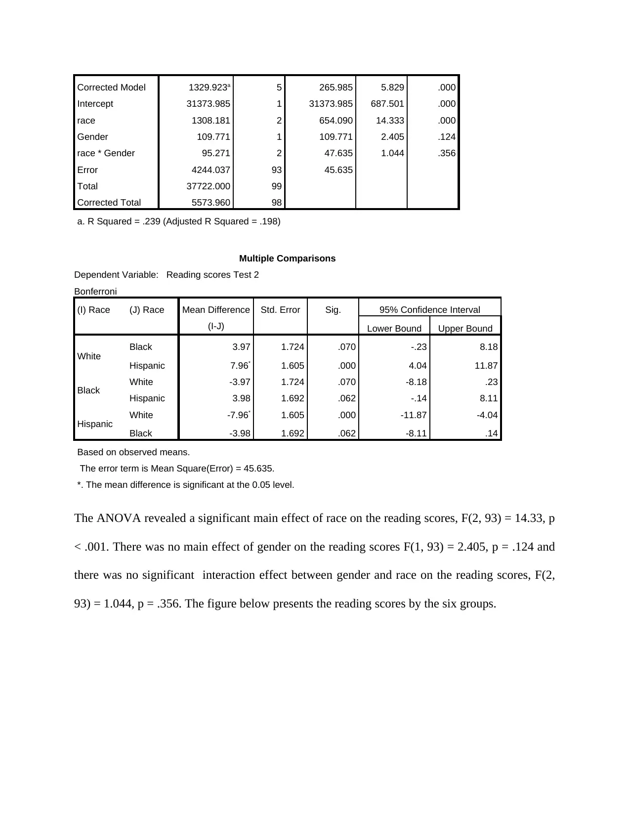
The ANOVA revealed a significant main effect of race on the reading scores, F(2, 93) = 14.33, p
< .001. There was no main effect of gender on the reading scores F(1, 93) = 2.405, p = .124 and
there was no significant interaction effect between gender and race on the reading scores, F(2,
93) = 1.044, p = .356. The figure below presents the reading scores by the six groups.

The above results therefore shows that our conclusions do not change or there are no additional
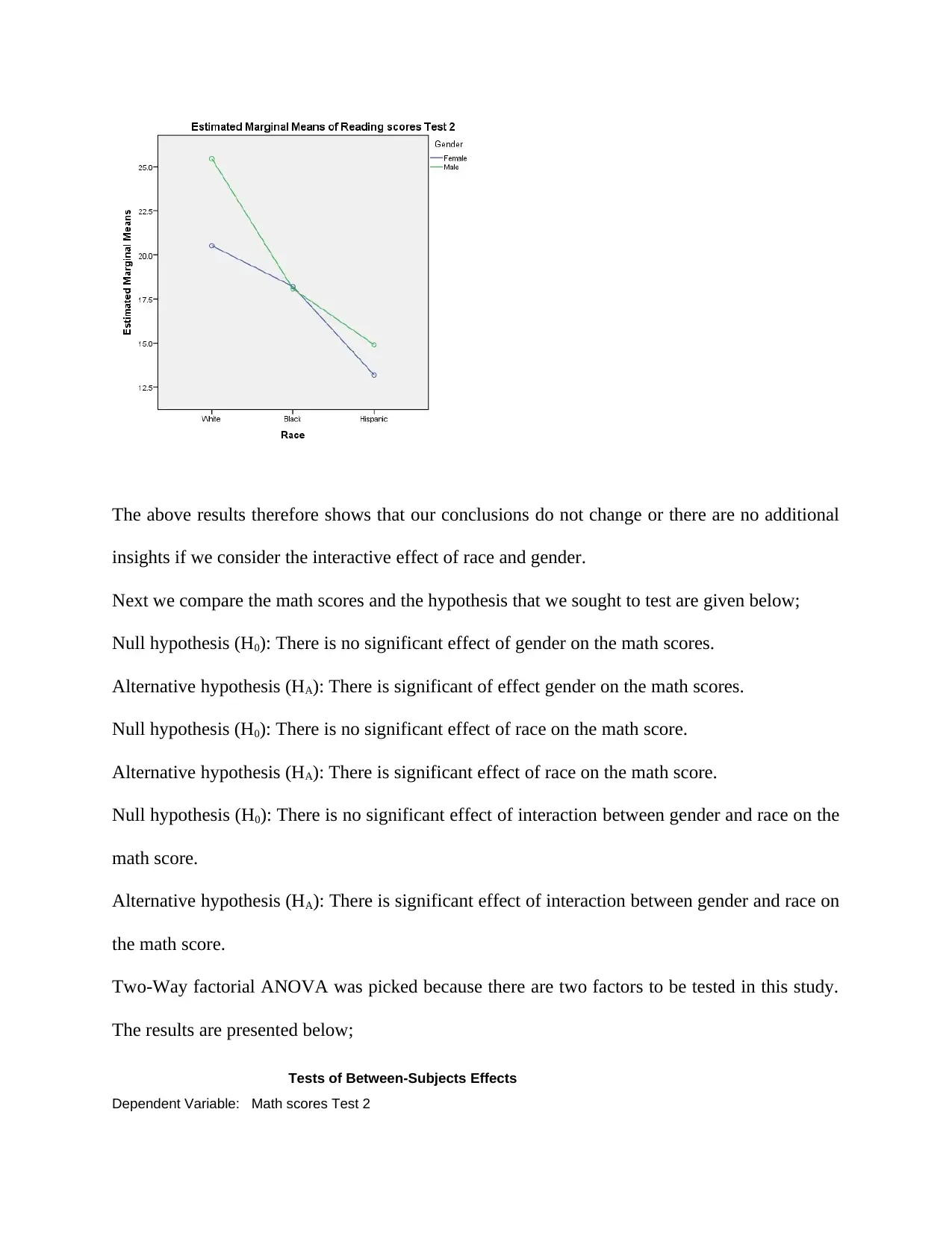
insights if we consider the interactive effect of race and gender.
Next we compare the math scores and the hypothesis that we sought to test are given below;
Null hypothesis (H0): There is no significant effect of gender on the math scores.
Alternative hypothesis (HA): There is significant of effect gender on the math scores.
Null hypothesis (H0): There is no significant effect of race on the math score.
Alternative hypothesis (HA): There is significant effect of race on the math score.
Null hypothesis (H0): There is no significant effect of interaction between gender and race on the
math score.
Alternative hypothesis (HA): There is significant effect of interaction between gender and race on
the math score.
Two-Way factorial ANOVA was picked because there are two factors to be tested in this study.
The results are presented below;
Tests of Between-Subjects Effects
Dependent Variable: Math scores Test 2

Source Type III Sum of
Squares
df Mean Square F Sig.
Corrected Model 1329.923a 5 265.985 5.829 .000
Intercept 24921.225 1 24921.225 546.101 .000
race 1308.181 2 654.090 14.333 .000
Gender 109.771 1 109.771 2.405 .124
race * Gender 95.271 2 47.635 1.044 .356
Error 4244.037 93 45.635
Total 30982.000 99
Corrected Total 5573.960 98
a. R Squared = .239 (Adjusted R Squared = .198)
Multiple Comparisons
Dependent Variable: Math scores Test 2
Bonferroni
(I) Race (J) Race Mean Difference
(I-J)
Std. Error Sig. 95% Confidence Interval
Lower Bound Upper Bound
White Black 3.97 1.724 .070 -.23 8.18
Hispanic 7.96* 1.605 .000 4.04 11.87
Black White -3.97 1.724 .070 -8.18 .23
Hispanic 3.98 1.692 .062 -.14 8.11
Hispanic White -7.96* 1.605 .000 -11.87 -4.04
Black -3.98 1.692 .062 -8.11 .14
Based on observed means.
The error term is Mean Square(Error) = 45.635.
*. The mean difference is significant at the .05 level.
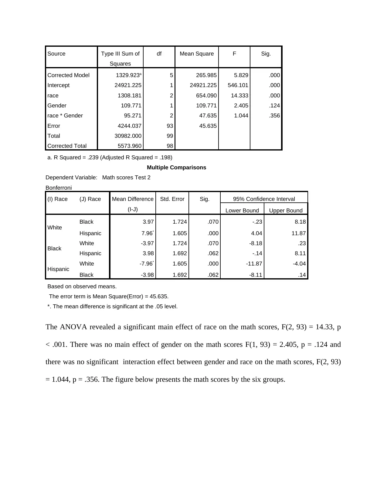
The ANOVA revealed a significant main effect of race on the math scores, F(2, 93) = 14.33, p
< .001. There was no main effect of gender on the math scores F(1, 93) = 2.405, p = .124 and
there was no significant interaction effect between gender and race on the math scores, F(2, 93)
= 1.044, p = .356. The figure below presents the math scores by the six groups.

The above results therefore shows that our conclusions do not change or there are no additional
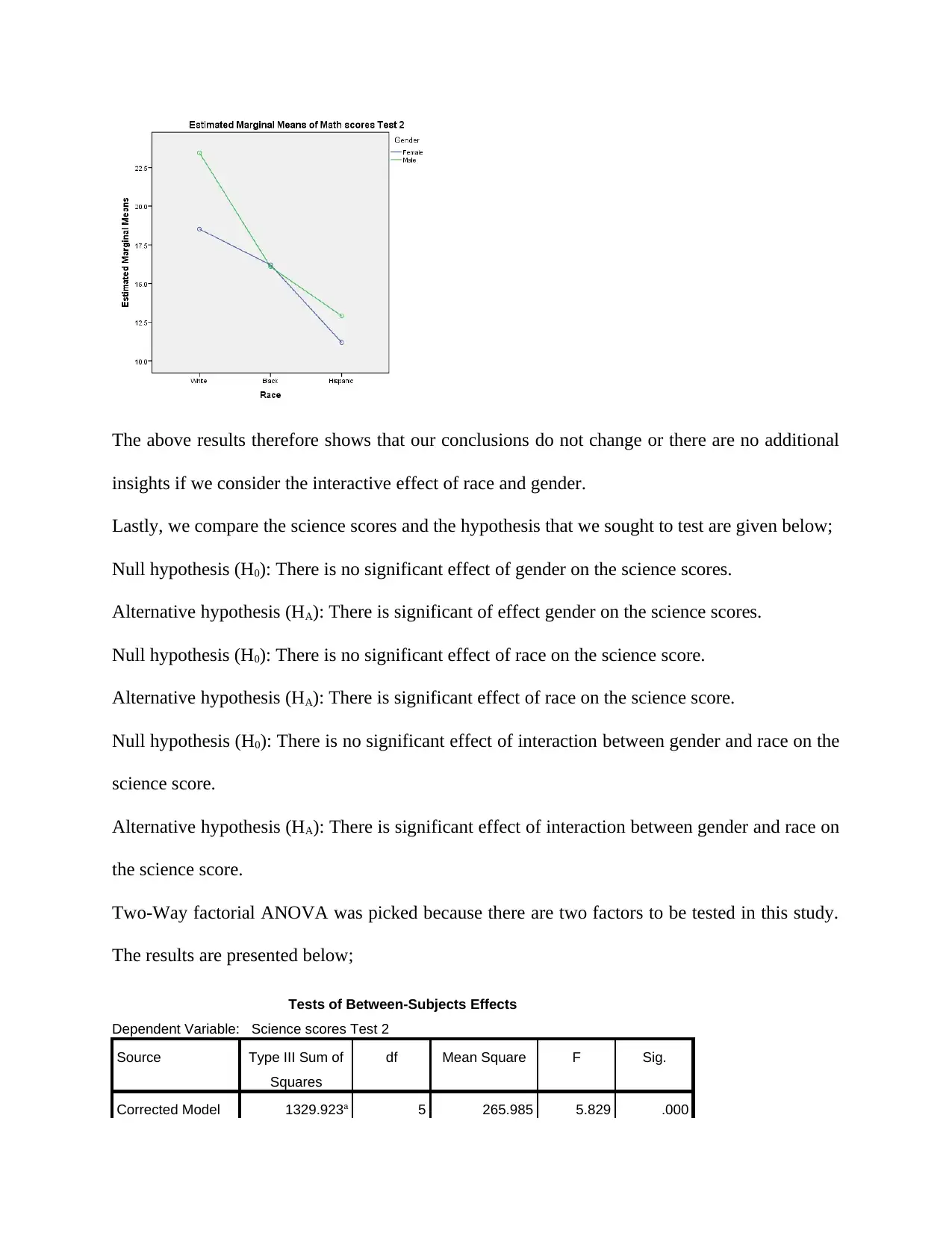
insights if we consider the interactive effect of race and gender.
Lastly, we compare the science scores and the hypothesis that we sought to test are given below;
Null hypothesis (H0): There is no significant effect of gender on the science scores.
Alternative hypothesis (HA): There is significant of effect gender on the science scores.
Null hypothesis (H0): There is no significant effect of race on the science score.
Alternative hypothesis (HA): There is significant effect of race on the science score.
Null hypothesis (H0): There is no significant effect of interaction between gender and race on the
science score.
Alternative hypothesis (HA): There is significant effect of interaction between gender and race on
the science score.
Two-Way factorial ANOVA was picked because there are two factors to be tested in this study.
The results are presented below;
Tests of Between-Subjects Effects
Dependent Variable: Science scores Test 2
Source Type III Sum of
Squares
df Mean Square F Sig.
Corrected Model 1329.923a 5 265.985 5.829 .000

Intercept 34878.647 1 34878.647 764.299 .000
race 1308.181 2 654.090 14.333 .000
Gender 109.771 1 109.771 2.405 .124
race * Gender 95.271 2 47.635 1.044 .356
Error 4244.037 93 45.635
Total 41389.000 99
Corrected Total 5573.960 98
a. R Squared = .239 (Adjusted R Squared = .198)
3. Race * Gender
Dependent Variable: Science scores Test 2
Race Gender Mean Std. Error 95% Confidence Interval
Lower Bound Upper Bound
White Female 21.522 1.409 18.725 24.319
Male 26.455 2.037 22.410 30.499
Black Female 19.200 1.744 15.736 22.664
Male 19.077 1.874 15.356 22.798
Hispanic Female 14.188 1.689 10.834 17.541
Male 15.905 1.474 12.977 18.832
The ANOVA revealed a significant main effect of race on the science scores, F(2, 93) = 14.33, p
< .001. There was no main effect of gender on the science scores F(1, 93) = 2.405, p = .124 and
there was no significant interaction effect between gender and race on the science scores, F(2,
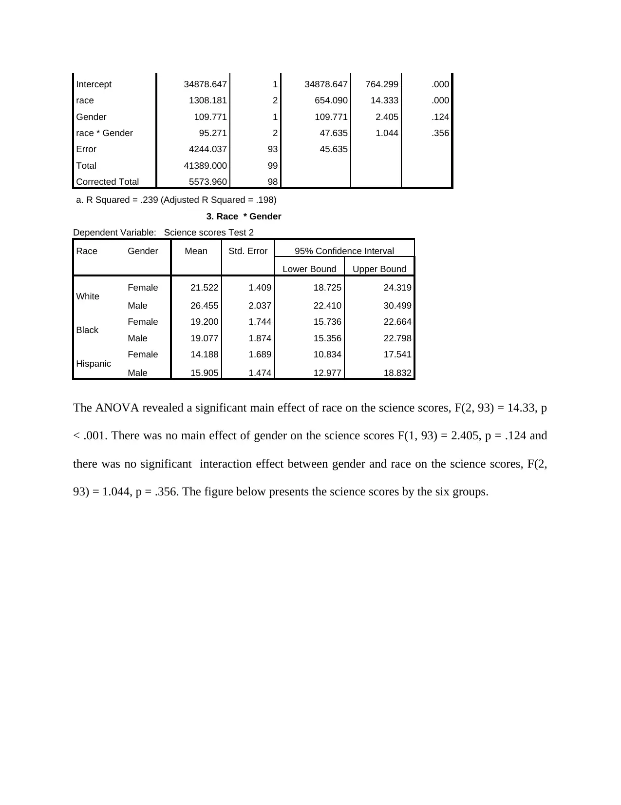
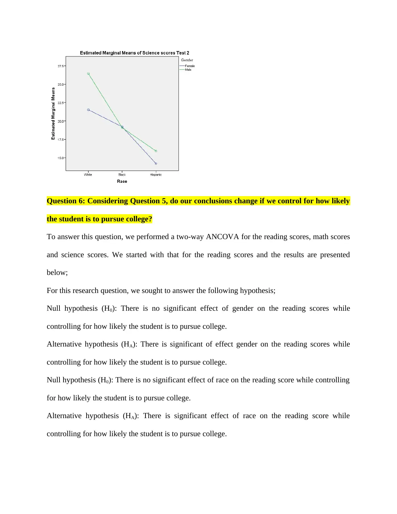
93) = 1.044, p = .356. The figure below presents the science scores by the six groups.

Question 6: Considering Question 5, do our conclusions change if we control for how likely
the student is to pursue college?
To answer this question, we performed a two-way ANCOVA for the reading scores, math scores
and science scores. We started with that for the reading scores and the results are presented
below;
For this research question, we sought to answer the following hypothesis;
Null hypothesis (H0): There is no significant effect of gender on the reading scores while
controlling for how likely the student is to pursue college.
Alternative hypothesis (HA): There is significant of effect gender on the reading scores while
controlling for how likely the student is to pursue college.
Null hypothesis (H0): There is no significant effect of race on the reading score while controlling
for how likely the student is to pursue college.
Alternative hypothesis (HA): There is significant effect of race on the reading score while
controlling for how likely the student is to pursue college.

Null hypothesis (H0): There is no significant effect of interaction between gender and race on the
reading score while controlling for how likely the student is to pursue college.
Alternative hypothesis (HA): There is significant effect of interaction between gender and race on
the reading score while controlling for how likely the student is to pursue college.
Two-Way factorial ANCOVA was picked because there are two factors to be tested in this study
and there is a control variable. The results are presented below;
Tests of Between-Subjects Effects
Dependent Variable: Reading scores Test 2
Source Type III Sum of
Squares
df Mean Square F Sig.
Corrected Model 1471.823a 6 245.304 5.502 .000
Intercept 2906.393 1 2906.393 65.183 .000
PlanColl 141.900 1 141.900 3.182 .078
race 1066.811 2 533.405 11.963 .000
Gender 71.068 1 71.068 1.594 .210
race * Gender 73.108 2 36.554 .820 .444
Error 4102.136 92 44.588
Total 37722.000 99
Corrected Total 5573.960 98
a. R Squared = .264 (Adjusted R Squared = .216)
ANCOVA results shows that there is a significant effect of race on the reading scores after
controlling for how likely the student is to pursue college, F(2, 92) = 11.963, p = 0.000. There
was however no significant effect of gender on the reading scores after controlling for how likely
the student is to pursue college, F(1, 92) = 1.594, p = 0.210. There was also no significant effect
of interaction between gender and race on the reading scores after controlling for how likely the
student is to pursue college, F(2, 92) = 0.820, p = 0.444.

The above results therefore shows that our conclusions do not change or there are no additional
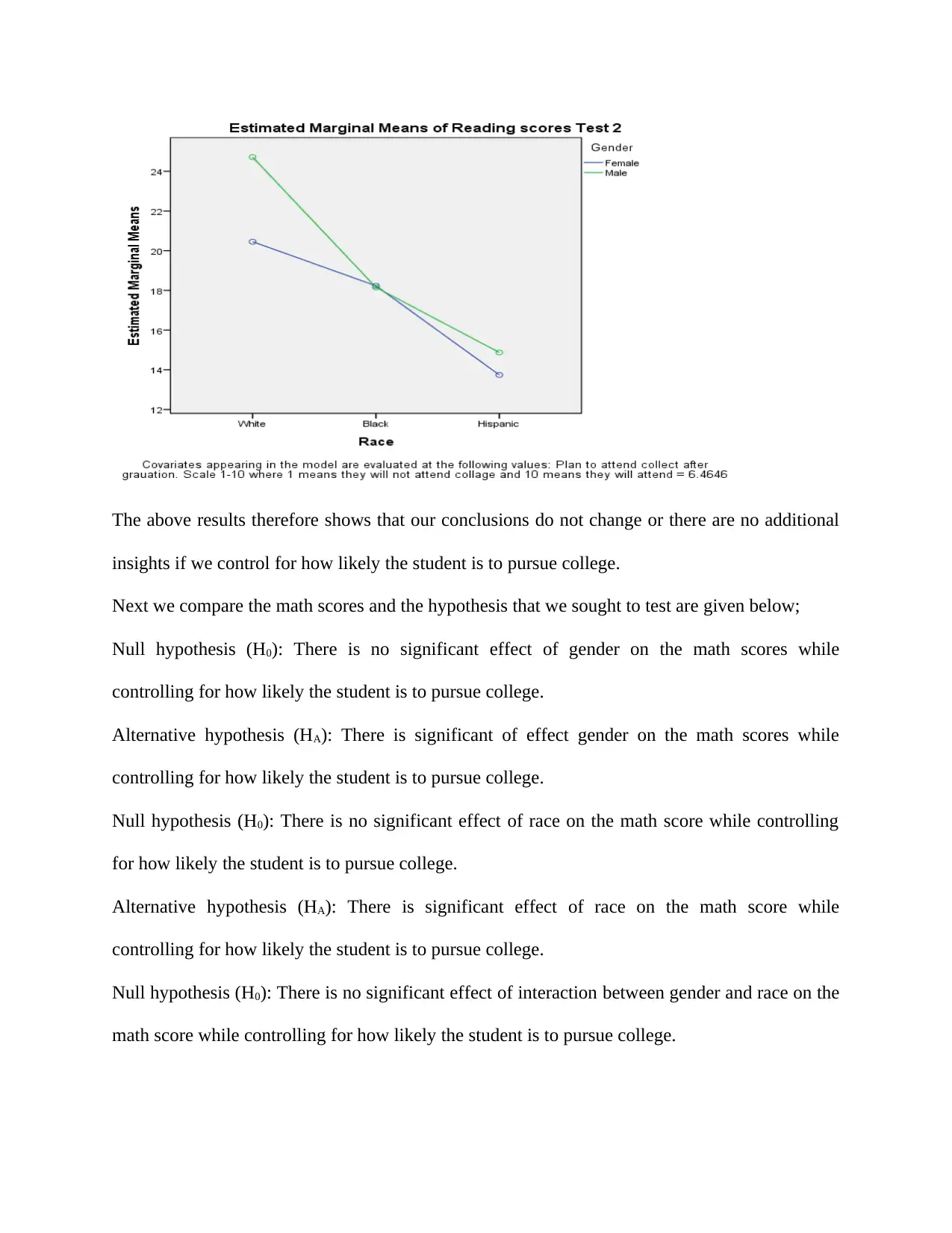
insights if we control for how likely the student is to pursue college.
Next we compare the math scores and the hypothesis that we sought to test are given below;
Null hypothesis (H0): There is no significant effect of gender on the math scores while
controlling for how likely the student is to pursue college.
Alternative hypothesis (HA): There is significant of effect gender on the math scores while
controlling for how likely the student is to pursue college.
Null hypothesis (H0): There is no significant effect of race on the math score while controlling
for how likely the student is to pursue college.
Alternative hypothesis (HA): There is significant effect of race on the math score while
controlling for how likely the student is to pursue college.
Null hypothesis (H0): There is no significant effect of interaction between gender and race on the
math score while controlling for how likely the student is to pursue college.

Alternative hypothesis (HA): There is significant effect of interaction between gender and race on
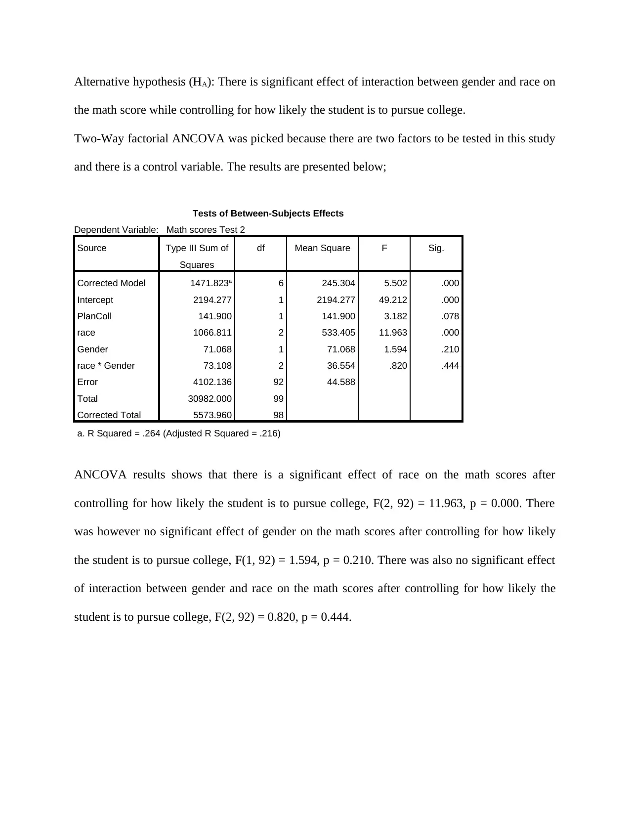
the math score while controlling for how likely the student is to pursue college.
Two-Way factorial ANCOVA was picked because there are two factors to be tested in this study
and there is a control variable. The results are presented below;
Tests of Between-Subjects Effects
Dependent Variable: Math scores Test 2
Source Type III Sum of
Squares
df Mean Square F Sig.
Corrected Model 1471.823a 6 245.304 5.502 .000
Intercept 2194.277 1 2194.277 49.212 .000
PlanColl 141.900 1 141.900 3.182 .078
race 1066.811 2 533.405 11.963 .000
Gender 71.068 1 71.068 1.594 .210
race * Gender 73.108 2 36.554 .820 .444
Error 4102.136 92 44.588
Total 30982.000 99
Corrected Total 5573.960 98
a. R Squared = .264 (Adjusted R Squared = .216)
ANCOVA results shows that there is a significant effect of race on the math scores after
controlling for how likely the student is to pursue college, F(2, 92) = 11.963, p = 0.000. There
was however no significant effect of gender on the math scores after controlling for how likely
the student is to pursue college, F(1, 92) = 1.594, p = 0.210. There was also no significant effect
of interaction between gender and race on the math scores after controlling for how likely the
student is to pursue college, F(2, 92) = 0.820, p = 0.444.

Lastly, we compare the science scores and the hypothesis that we sought to test are given below;
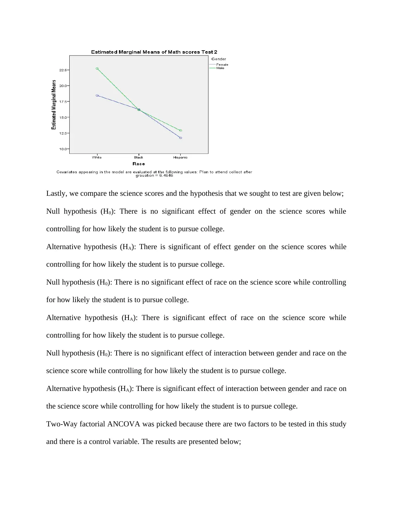
Null hypothesis (H0): There is no significant effect of gender on the science scores while
controlling for how likely the student is to pursue college.
Alternative hypothesis (HA): There is significant of effect gender on the science scores while
controlling for how likely the student is to pursue college.
Null hypothesis (H0): There is no significant effect of race on the science score while controlling
for how likely the student is to pursue college.
Alternative hypothesis (HA): There is significant effect of race on the science score while
controlling for how likely the student is to pursue college.
Null hypothesis (H0): There is no significant effect of interaction between gender and race on the
science score while controlling for how likely the student is to pursue college.
Alternative hypothesis (HA): There is significant effect of interaction between gender and race on
the science score while controlling for how likely the student is to pursue college.
Two-Way factorial ANCOVA was picked because there are two factors to be tested in this study
and there is a control variable. The results are presented below;

Tests of Between-Subjects Effects
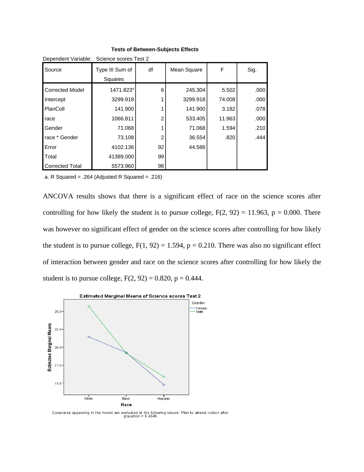
Dependent Variable: Science scores Test 2
Source Type III Sum of
Squares
df Mean Square F Sig.
Corrected Model 1471.823a 6 245.304 5.502 .000
Intercept 3299.918 1 3299.918 74.008 .000
PlanColl 141.900 1 141.900 3.182 .078
race 1066.811 2 533.405 11.963 .000
Gender 71.068 1 71.068 1.594 .210
race * Gender 73.108 2 36.554 .820 .444
Error 4102.136 92 44.588
Total 41389.000 99
Corrected Total 5573.960 98
a. R Squared = .264 (Adjusted R Squared = .216)
ANCOVA results shows that there is a significant effect of race on the science scores after
controlling for how likely the student is to pursue college, F(2, 92) = 11.963, p = 0.000. There
was however no significant effect of gender on the science scores after controlling for how likely
the student is to pursue college, F(1, 92) = 1.594, p = 0.210. There was also no significant effect
of interaction between gender and race on the science scores after controlling for how likely the
student is to pursue college, F(2, 92) = 0.820, p = 0.444.

Question 7: Test the three assumptions proposed in the above paragraph. The variable
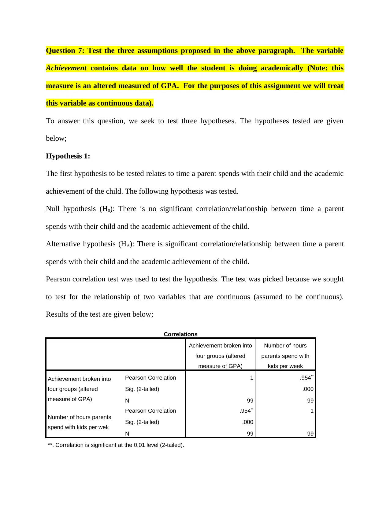
Achievement contains data on how well the student is doing academically (Note: this
measure is an altered measured of GPA. For the purposes of this assignment we will treat
this variable as continuous data).
To answer this question, we seek to test three hypotheses. The hypotheses tested are given
below;
Hypothesis 1:
The first hypothesis to be tested relates to time a parent spends with their child and the academic
achievement of the child. The following hypothesis was tested.
Null hypothesis (H0): There is no significant correlation/relationship between time a parent
spends with their child and the academic achievement of the child.
Alternative hypothesis (HA): There is significant correlation/relationship between time a parent
spends with their child and the academic achievement of the child.
Pearson correlation test was used to test the hypothesis. The test was picked because we sought
to test for the relationship of two variables that are continuous (assumed to be continuous).
Results of the test are given below;
Correlations
Achievement broken into
four groups (altered
measure of GPA)
Number of hours
parents spend with
kids per week
Achievement broken into
four groups (altered
measure of GPA)
Pearson Correlation 1 .954**
Sig. (2-tailed) .000
N 99 99
Number of hours parents
spend with kids per wek
Pearson Correlation .954** 1
Sig. (2-tailed) .000
N 99 99
**. Correlation is significant at the 0.01 level (2-tailed).

A Pearson product-moment correlation coefficient was computed to assess the relationship
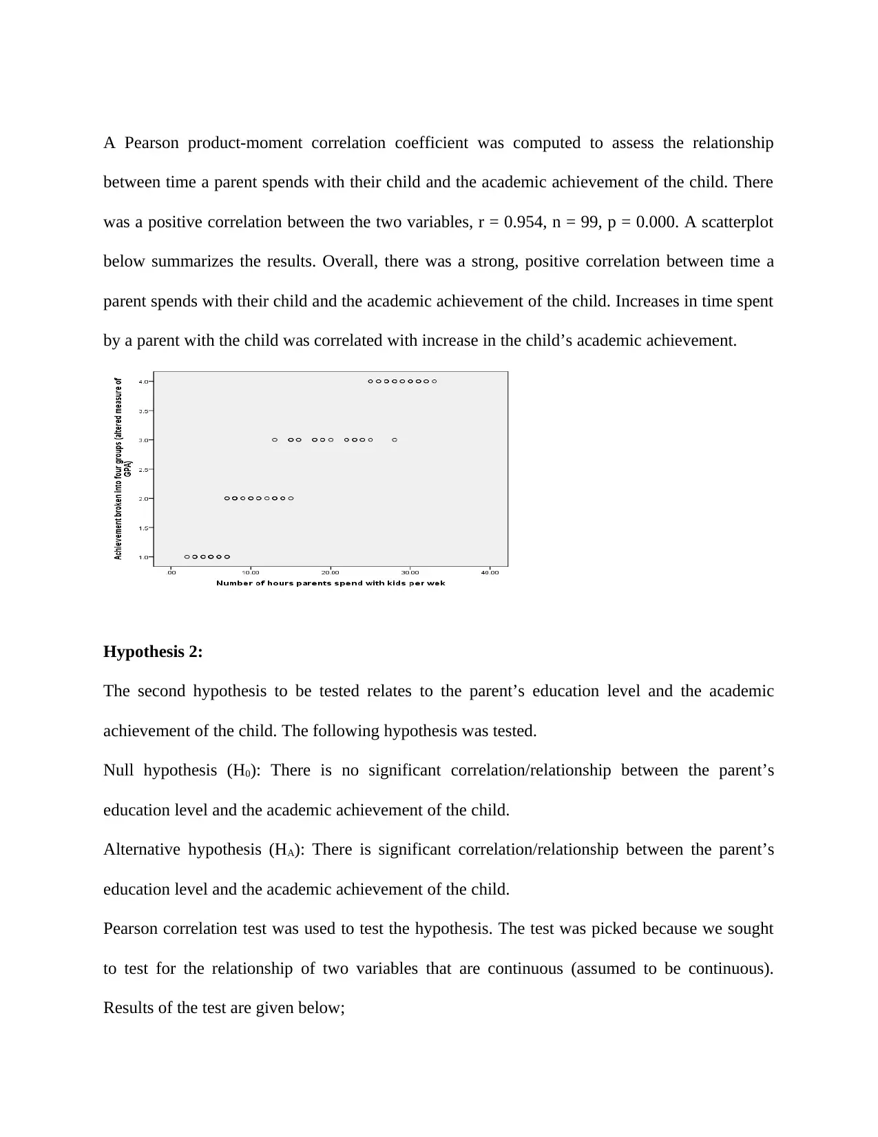
between time a parent spends with their child and the academic achievement of the child. There
was a positive correlation between the two variables, r = 0.954, n = 99, p = 0.000. A scatterplot
below summarizes the results. Overall, there was a strong, positive correlation between time a
parent spends with their child and the academic achievement of the child. Increases in time spent
by a parent with the child was correlated with increase in the child’s academic achievement.
Hypothesis 2:
The second hypothesis to be tested relates to the parent’s education level and the academic
achievement of the child. The following hypothesis was tested.
Null hypothesis (H0): There is no significant correlation/relationship between the parent’s
education level and the academic achievement of the child.
Alternative hypothesis (HA): There is significant correlation/relationship between the parent’s
education level and the academic achievement of the child.
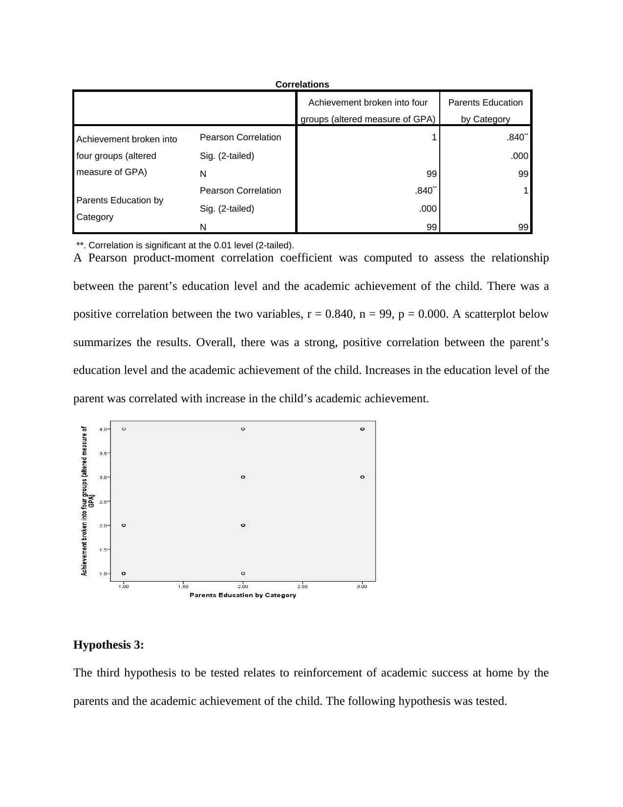
Pearson correlation test was used to test the hypothesis. The test was picked because we sought
to test for the relationship of two variables that are continuous (assumed to be continuous).
Results of the test are given below;

Correlations
Achievement broken into four
groups (altered measure of GPA)
Parents Education
by Category
Achievement broken into
four groups (altered
measure of GPA)
Pearson Correlation 1 .840**
Sig. (2-tailed) .000
N 99 99
Parents Education by
Category
Pearson Correlation .840** 1
Sig. (2-tailed) .000
N 99 99
**. Correlation is significant at the 0.01 level (2-tailed).
A Pearson product-moment correlation coefficient was computed to assess the relationship
between the parent’s education level and the academic achievement of the child. There was a
positive correlation between the two variables, r = 0.840, n = 99, p = 0.000. A scatterplot below
summarizes the results. Overall, there was a strong, positive correlation between the parent’s
education level and the academic achievement of the child. Increases in the education level of the
parent was correlated with increase in the child’s academic achievement.
Hypothesis 3:
The third hypothesis to be tested relates to reinforcement of academic success at home by the
parents and the academic achievement of the child. The following hypothesis was tested.

Null hypothesis (H0): There is no significant difference in the academic achievement between
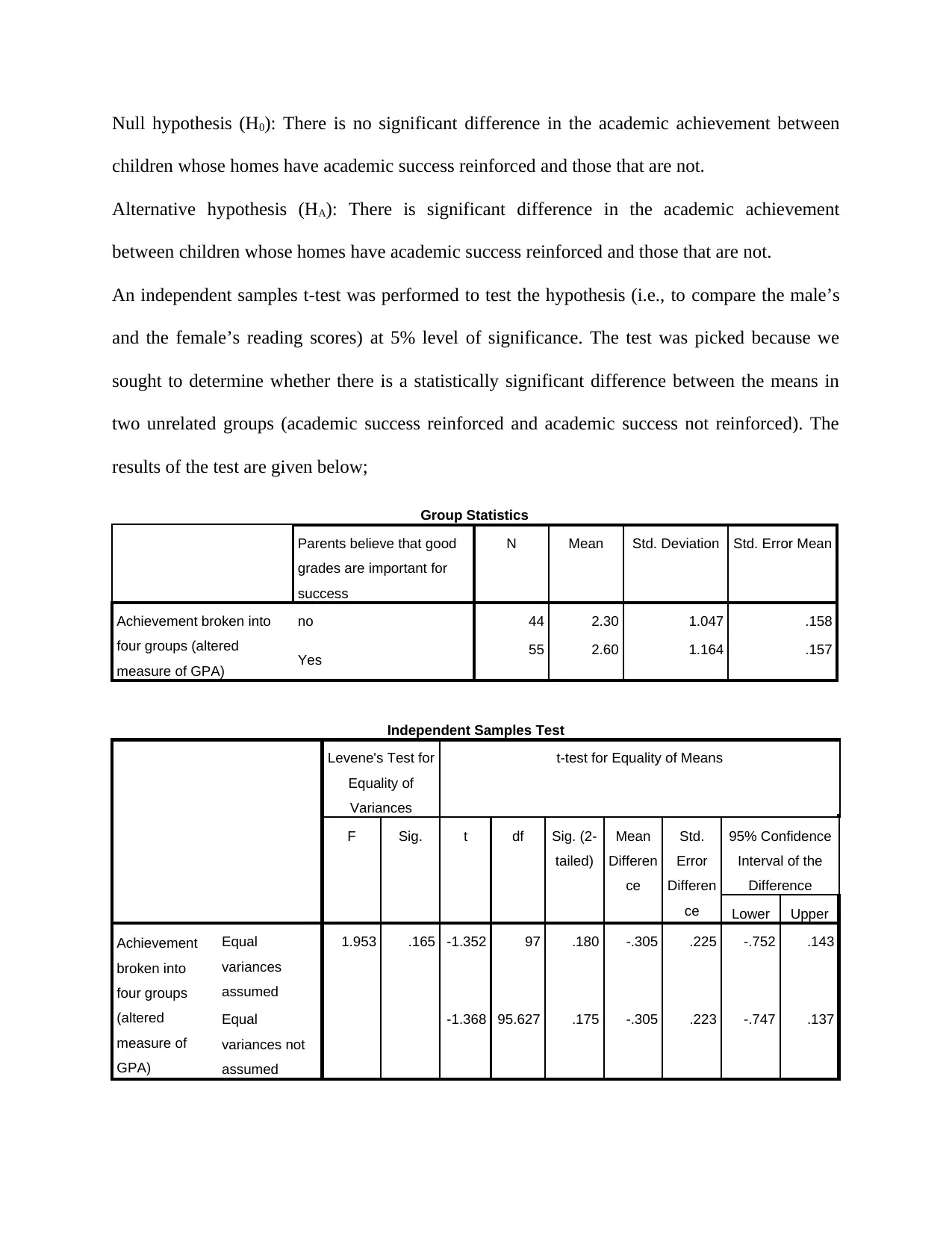
children whose homes have academic success reinforced and those that are not.
Alternative hypothesis (HA): There is significant difference in the academic achievement
between children whose homes have academic success reinforced and those that are not.
An independent samples t-test was performed to test the hypothesis (i.e., to compare the male’s
and the female’s reading scores) at 5% level of significance. The test was picked because we
sought to determine whether there is a statistically significant difference between the means in
two unrelated groups (academic success reinforced and academic success not reinforced). The
results of the test are given below;
Group Statistics
Parents believe that good
grades are important for
success
N Mean Std. Deviation Std. Error Mean
Achievement broken into
four groups (altered
measure of GPA)
no 44 2.30 1.047 .158
Yes 55 2.60 1.164 .157
Independent Samples Test
Levene's Test for
Equality of
Variances
t-test for Equality of Means
F Sig. t df Sig. (2-
tailed)
Mean
Differen
ce
Std.
Error
Differen
ce
95% Confidence
Interval of the
Difference
Lower Upper
Achievement
broken into
four groups
(altered
measure of
GPA)
Equal
variances
assumed
1.953 .165 -1.352 97 .180 -.305 .225 -.752 .143
Equal
variances not
assumed
-1.368 95.627 .175 -.305 .223 -.747 .137

Results showed that the students where there is no reinforcement of academic success at their
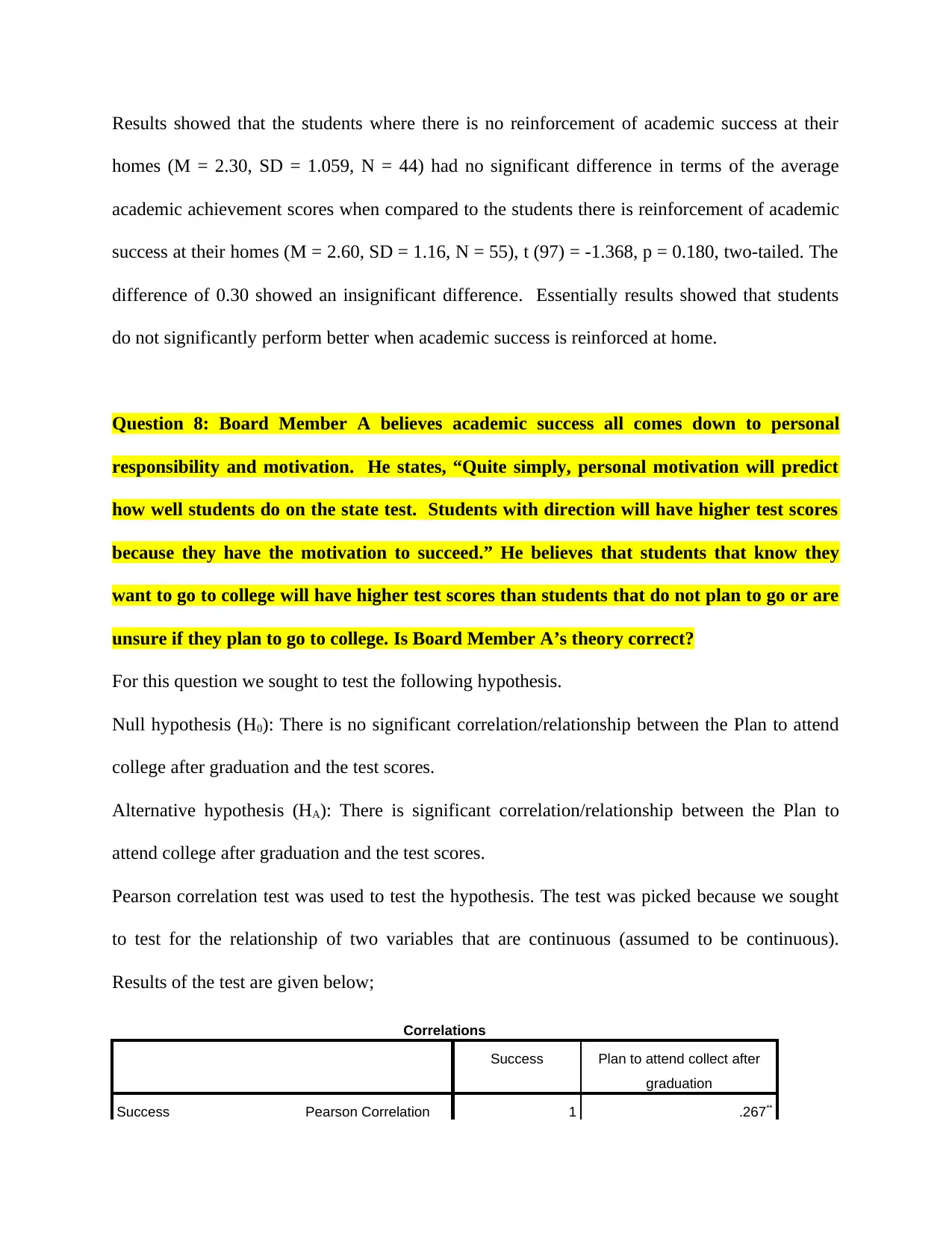
homes (M = 2.30, SD = 1.059, N = 44) had no significant difference in terms of the average
academic achievement scores when compared to the students there is reinforcement of academic
success at their homes (M = 2.60, SD = 1.16, N = 55), t (97) = -1.368, p = 0.180, two-tailed. The
difference of 0.30 showed an insignificant difference. Essentially results showed that students
do not significantly perform better when academic success is reinforced at home.
Question 8: Board Member A believes academic success all comes down to personal
responsibility and motivation. He states, “Quite simply, personal motivation will predict
how well students do on the state test. Students with direction will have higher test scores
because they have the motivation to succeed.” He believes that students that know they
want to go to college will have higher test scores than students that do not plan to go or are
unsure if they plan to go to college. Is Board Member A’s theory correct?
For this question we sought to test the following hypothesis.
Null hypothesis (H0): There is no significant correlation/relationship between the Plan to attend
college after graduation and the test scores.
Alternative hypothesis (HA): There is significant correlation/relationship between the Plan to
attend college after graduation and the test scores.
Pearson correlation test was used to test the hypothesis. The test was picked because we sought
to test for the relationship of two variables that are continuous (assumed to be continuous).
Results of the test are given below;
Correlations
Success Plan to attend collect after
graduation
Success Pearson Correlation 1 .267**

Sig. (2-tailed) .007
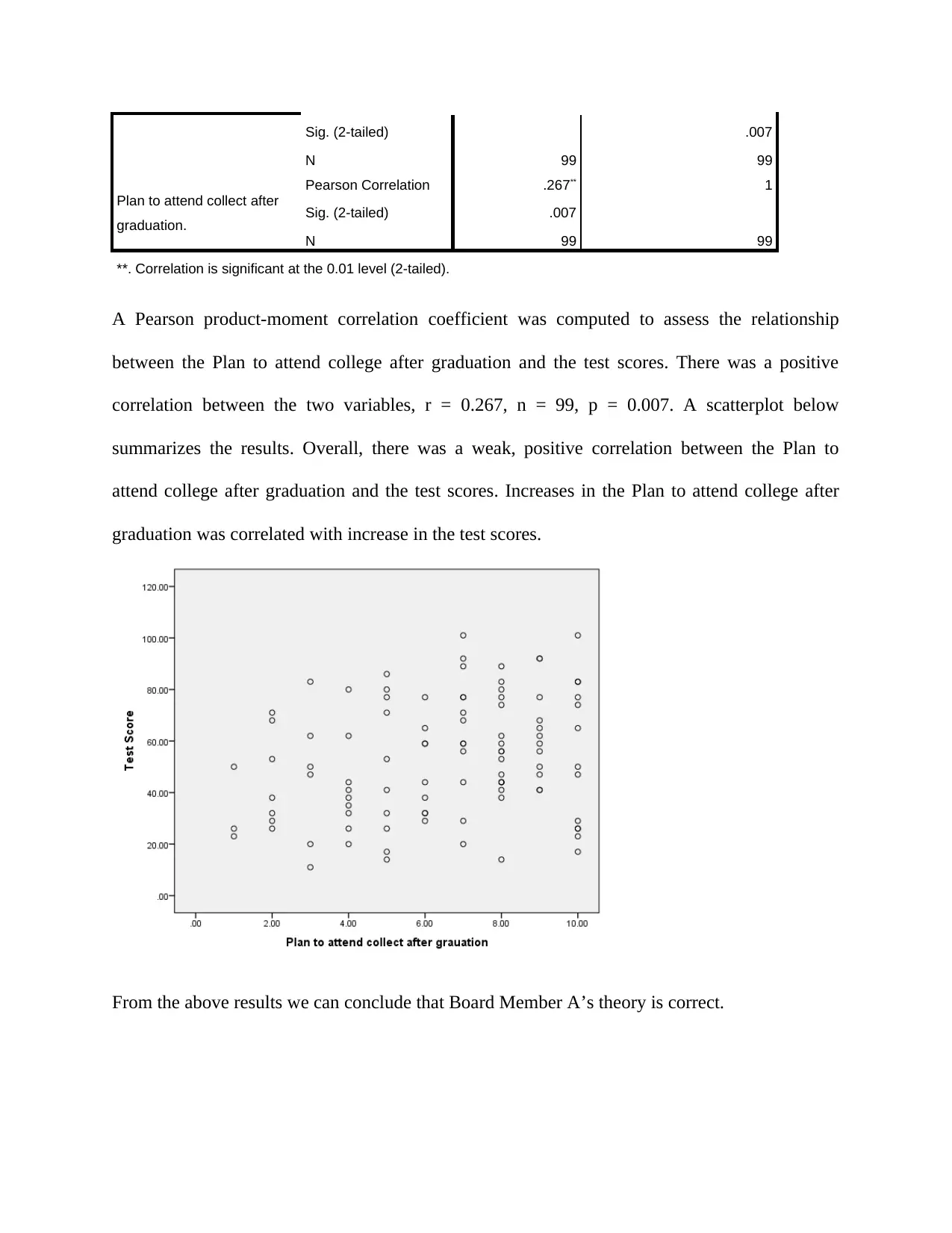
N 99 99
Plan to attend collect after
graduation.
Pearson Correlation .267** 1
Sig. (2-tailed) .007
N 99 99
**. Correlation is significant at the 0.01 level (2-tailed).
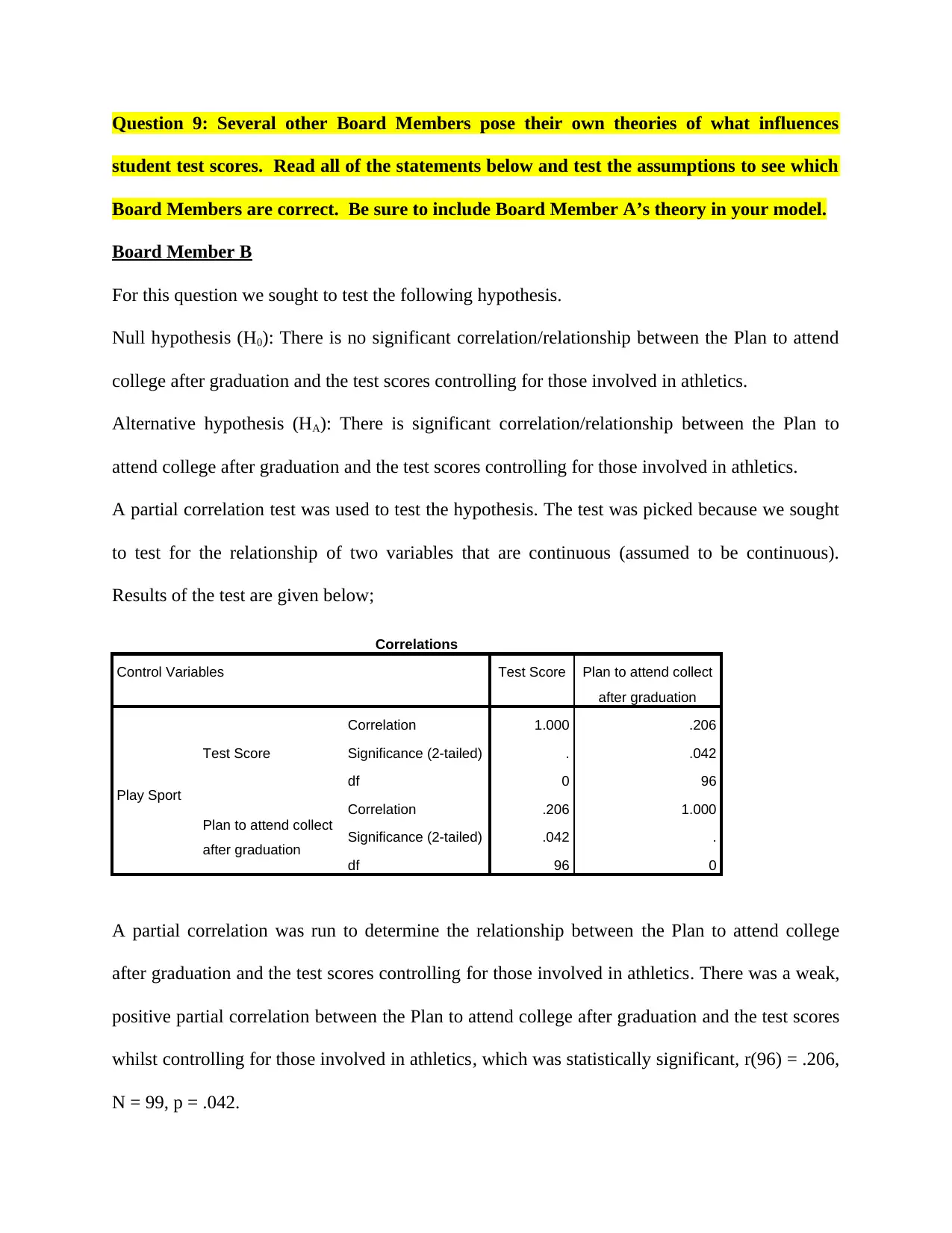
A Pearson product-moment correlation coefficient was computed to assess the relationship
between the Plan to attend college after graduation and the test scores. There was a positive
correlation between the two variables, r = 0.267, n = 99, p = 0.007. A scatterplot below
summarizes the results. Overall, there was a weak, positive correlation between the Plan to
attend college after graduation and the test scores. Increases in the Plan to attend college after
graduation was correlated with increase in the test scores.
From the above results we can conclude that Board Member A’s theory is correct.

Question 9: Several other Board Members pose their own theories of what influences
student test scores. Read all of the statements below and test the assumptions to see which
Board Members are correct. Be sure to include Board Member A’s theory in your model.
Board Member B
For this question we sought to test the following hypothesis.
Null hypothesis (H0): There is no significant correlation/relationship between the Plan to attend
college after graduation and the test scores controlling for those involved in athletics.
Alternative hypothesis (HA): There is significant correlation/relationship between the Plan to
attend college after graduation and the test scores controlling for those involved in athletics.
A partial correlation test was used to test the hypothesis. The test was picked because we sought
to test for the relationship of two variables that are continuous (assumed to be continuous).
Results of the test are given below;
Correlations
Control Variables Test Score Plan to attend collect
after graduation
Play Sport
Test Score
Correlation 1.000 .206
Significance (2-tailed) . .042
df 0 96
Plan to attend collect
after graduation
Correlation .206 1.000
Significance (2-tailed) .042 .
df 96 0
A partial correlation was run to determine the relationship between the Plan to attend college
after graduation and the test scores controlling for those involved in athletics. There was a weak,
positive partial correlation between the Plan to attend college after graduation and the test scores
whilst controlling for those involved in athletics, which was statistically significant, r(96) = .206,
N = 99, p = .042.

Board Member C
For this question we sought to test the following hypothesis.
Null hypothesis (H0): There is no significant correlation/relationship between the Plan to attend
college after graduation and the test scores controlling for those involved in athletics and parents
who value education.
Alternative hypothesis (HA): There is significant correlation/relationship between the Plan to
attend college after graduation and the test scores controlling for those involved in athletics and
parents who value education.
A partial correlation test was used to test the hypothesis. The test was picked because we sought
to test for the relationship of two variables that are continuous (assumed to be continuous).
Results of the test are given below;
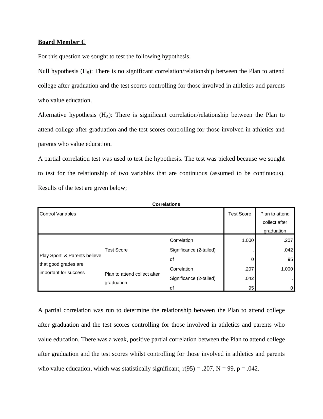
Correlations
Control Variables Test Score Plan to attend
collect after
graduation
Play Sport & Parents believe
that good grades are
important for success
Test Score
Correlation 1.000 .207
Significance (2-tailed) . .042
df 0 95
Plan to attend collect after
graduation
Correlation .207 1.000
Significance (2-tailed) .042 .
df 95 0
A partial correlation was run to determine the relationship between the Plan to attend college
after graduation and the test scores controlling for those involved in athletics and parents who
value education. There was a weak, positive partial correlation between the Plan to attend college
after graduation and the test scores whilst controlling for those involved in athletics and parents
who value education, which was statistically significant, r(95) = .207, N = 99, p = .042.

Board Member D
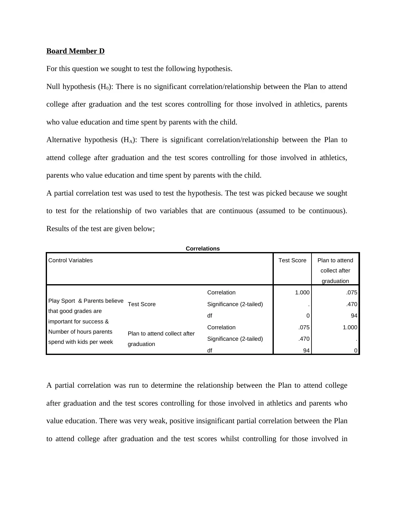
For this question we sought to test the following hypothesis.
Null hypothesis (H0): There is no significant correlation/relationship between the Plan to attend
college after graduation and the test scores controlling for those involved in athletics, parents
who value education and time spent by parents with the child.
Alternative hypothesis (HA): There is significant correlation/relationship between the Plan to
attend college after graduation and the test scores controlling for those involved in athletics,
parents who value education and time spent by parents with the child.
A partial correlation test was used to test the hypothesis. The test was picked because we sought
to test for the relationship of two variables that are continuous (assumed to be continuous).
Results of the test are given below;
Correlations
Control Variables Test Score Plan to attend
collect after
graduation
Play Sport & Parents believe
that good grades are
important for success &
Number of hours parents
spend with kids per week
Test Score
Correlation 1.000 .075
Significance (2-tailed) . .470
df 0 94
Plan to attend collect after
graduation
Correlation .075 1.000
Significance (2-tailed) .470 .
df 94 0
A partial correlation was run to determine the relationship between the Plan to attend college
after graduation and the test scores controlling for those involved in athletics and parents who
value education. There was very weak, positive insignificant partial correlation between the Plan
to attend college after graduation and the test scores whilst controlling for those involved in

athletics, parents who value education and time spent by parents with the child, r(94) = .075, N =
99, p = .470.
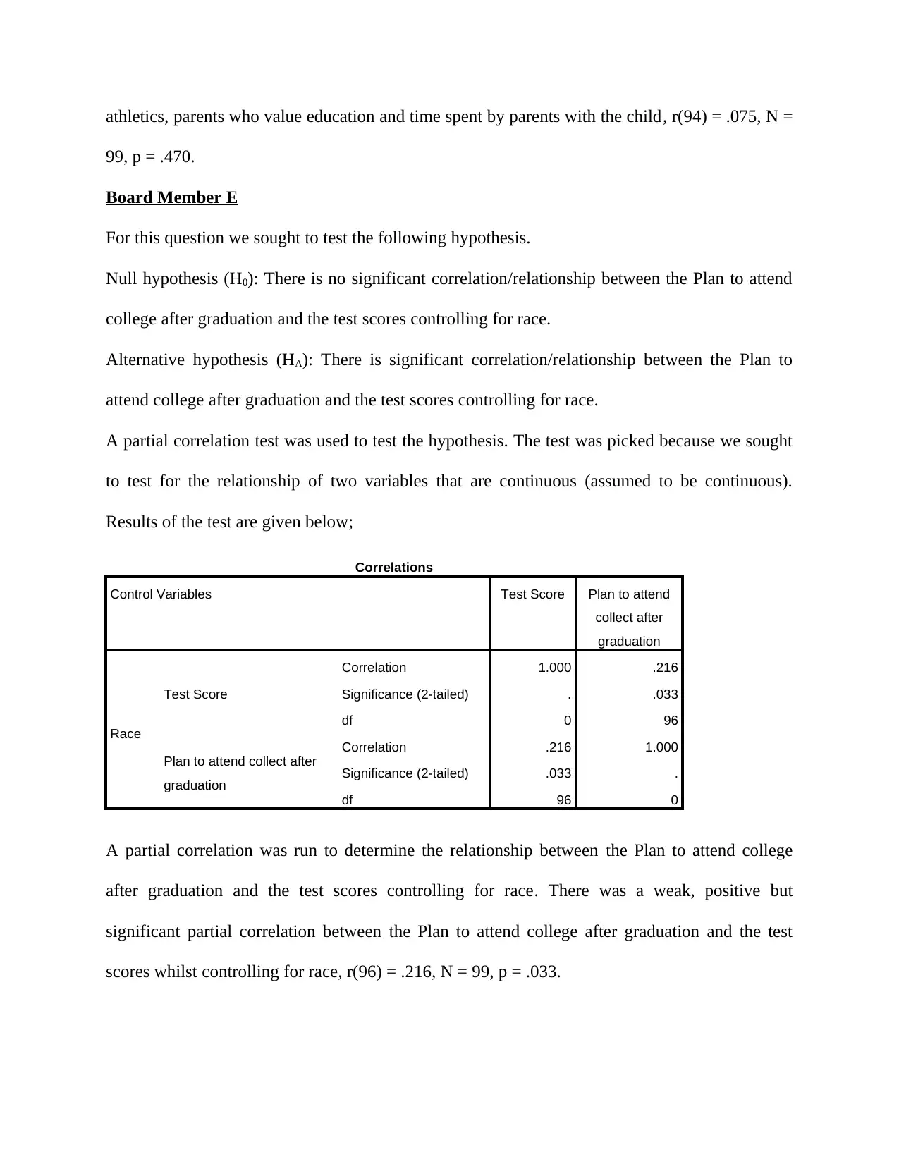
Board Member E
For this question we sought to test the following hypothesis.
Null hypothesis (H0): There is no significant correlation/relationship between the Plan to attend
college after graduation and the test scores controlling for race.
Alternative hypothesis (HA): There is significant correlation/relationship between the Plan to
attend college after graduation and the test scores controlling for race.
A partial correlation test was used to test the hypothesis. The test was picked because we sought
to test for the relationship of two variables that are continuous (assumed to be continuous).
Results of the test are given below;
Correlations
Control Variables Test Score Plan to attend
collect after
graduation
Race
Test Score
Correlation 1.000 .216
Significance (2-tailed) . .033
df 0 96
Plan to attend collect after
graduation
Correlation .216 1.000
Significance (2-tailed) .033 .
df 96 0
A partial correlation was run to determine the relationship between the Plan to attend college
after graduation and the test scores controlling for race. There was a weak, positive but
significant partial correlation between the Plan to attend college after graduation and the test
scores whilst controlling for race, r(96) = .216, N = 99, p = .033.

Board Member F
For this question we sought to test the following hypothesis.
Null hypothesis (H0): There is no significant correlation/relationship between amount of time
spent studying at home and the test scores.
Alternative hypothesis (HA): There is significant correlation/relationship between amount of time
spent studying at home and the test scores.
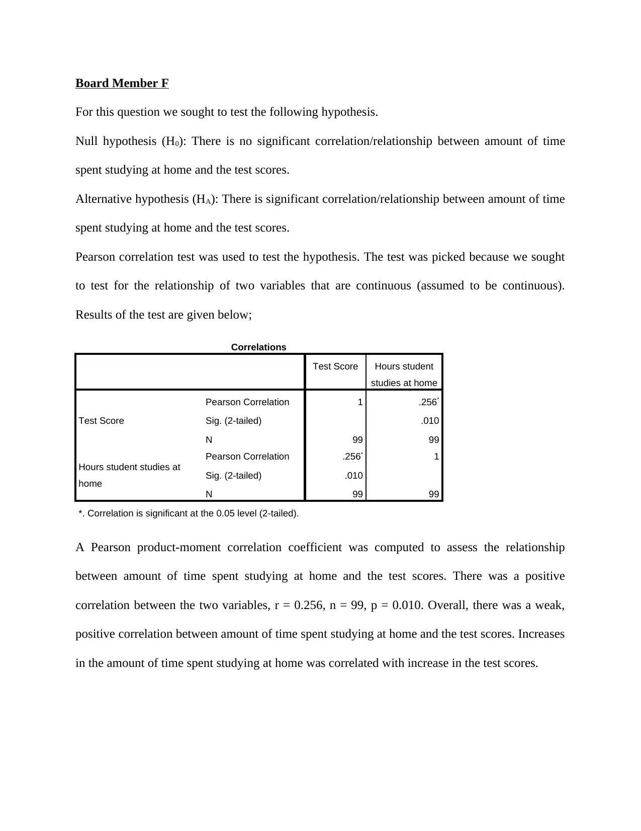
Pearson correlation test was used to test the hypothesis. The test was picked because we sought
to test for the relationship of two variables that are continuous (assumed to be continuous).
Results of the test are given below;
Correlations
Test Score Hours student
studies at home
Test Score
Pearson Correlation 1 .256*
Sig. (2-tailed) .010
N 99 99
Hours student studies at
home
Pearson Correlation .256* 1
Sig. (2-tailed) .010
N 99 99
*. Correlation is significant at the 0.05 level (2-tailed).
A Pearson product-moment correlation coefficient was computed to assess the relationship
between amount of time spent studying at home and the test scores. There was a positive
correlation between the two variables, r = 0.256, n = 99, p = 0.010. Overall, there was a weak,
positive correlation between amount of time spent studying at home and the test scores. Increases
in the amount of time spent studying at home was correlated with increase in the test scores.

Question 10: Board Member G
For this question we sought to test the following hypothesis.
Null hypothesis (H0): There is no significant correlation/relationship between amount of time
spent studying at home and the test scores.
Alternative hypothesis (HA): There is significant correlation/relationship between amount of time
spent studying at home and the test scores.
Null hypothesis (H0): There is no significant correlation/relationship between number of times
attended afterschool program and the test scores.
Alternative hypothesis (HA): There is significant correlation/relationship between number of
times attended afterschool program and the test scores.
Pearson correlation test was used to test the hypothesis. The test was picked because we sought
to test for the relationship of two variables that are continuous (assumed to be continuous).
Results of the test are given below;
Correlations
Test
Score
Hours student
studies at home
Number of times student
attended afterschool program

Test Score
Pearson Correlation 1 .256* .965**
Sig. (2-tailed) .010 .000
N 99 99 99
Hours student studies
at home
Pearson Correlation .256* 1 .263**
Sig. (2-tailed) .010 .009
N 99 99 99
Number of times
student attended
afterschool program
Pearson Correlation .965** .263** 1
Sig. (2-tailed) .000 .009
N 99 99 99
*. Correlation is significant at the 0.05 level (2-tailed).
**. Correlation is significant at the 0.01 level (2-tailed).
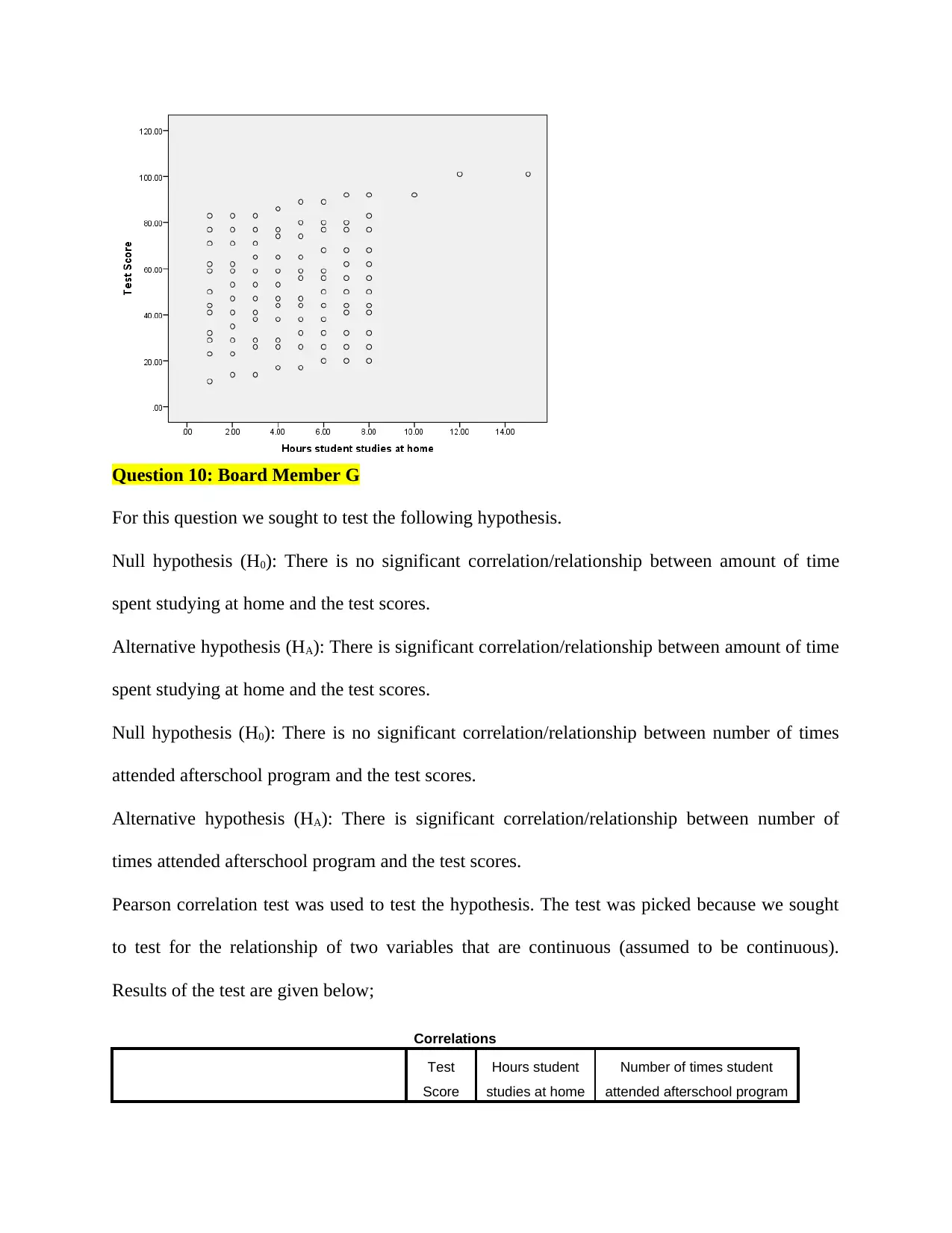
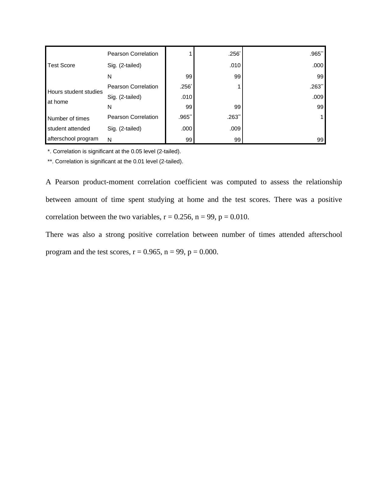
A Pearson product-moment correlation coefficient was computed to assess the relationship
between amount of time spent studying at home and the test scores. There was a positive
correlation between the two variables, r = 0.256, n = 99, p = 0.010.
There was also a strong positive correlation between number of times attended afterschool
program and the test scores, r = 0.965, n = 99, p = 0.000.