STA 510 Business Statistics - Assignment

STA 510 Business Statistics
Semester 1, 2018
Assignment 2
Solution
Question 2
a)
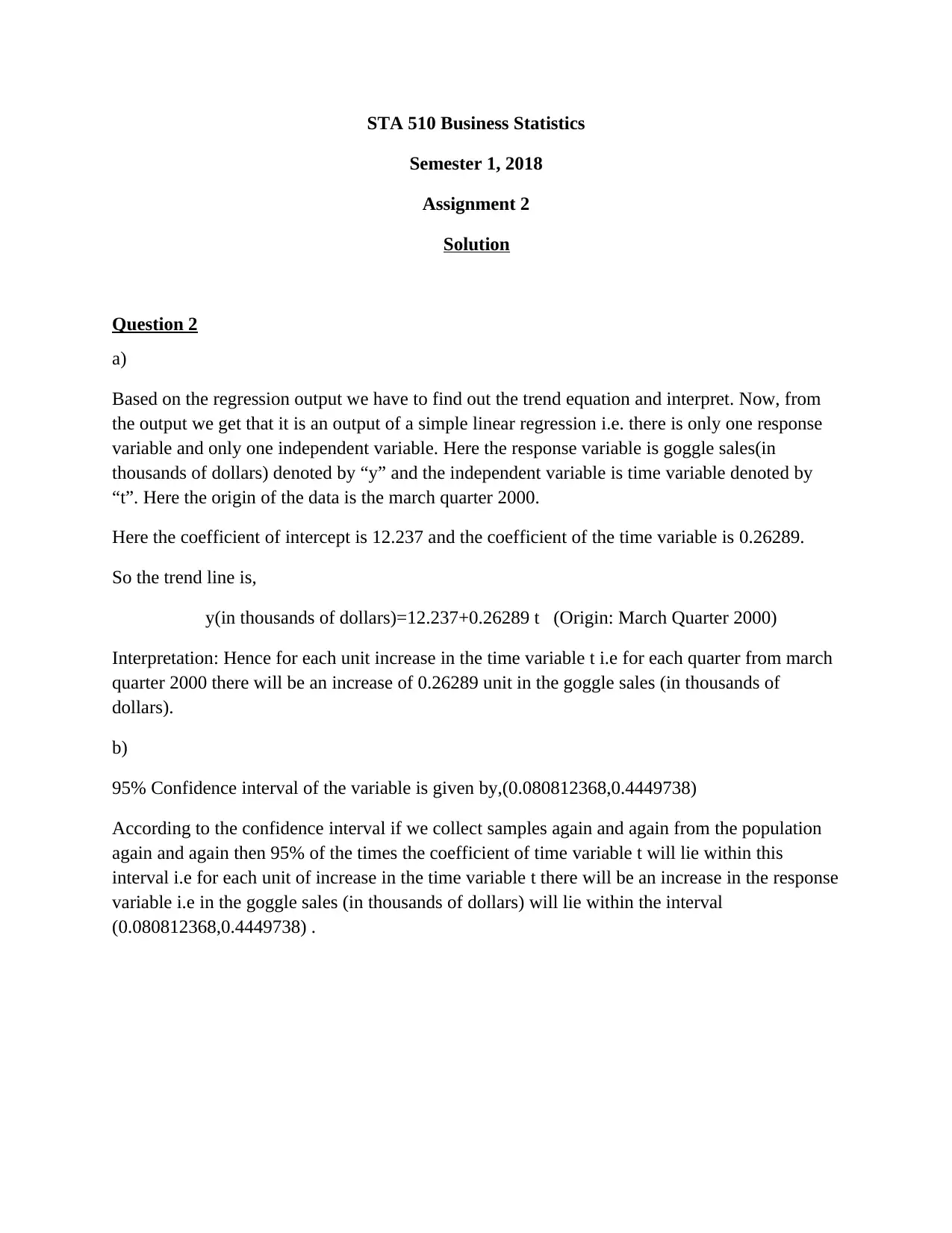
Based on the regression output we have to find out the trend equation and interpret. Now, from
the output we get that it is an output of a simple linear regression i.e. there is only one response
variable and only one independent variable. Here the response variable is goggle sales(in
thousands of dollars) denoted by “y” and the independent variable is time variable denoted by
“t”. Here the origin of the data is the march quarter 2000.
Here the coefficient of intercept is 12.237 and the coefficient of the time variable is 0.26289.
So the trend line is,
y(in thousands of dollars)=12.237+0.26289 t (Origin: March Quarter 2000)
Interpretation: Hence for each unit increase in the time variable t i.e for each quarter from march
quarter 2000 there will be an increase of 0.26289 unit in the goggle sales (in thousands of
dollars).
b)
95% Confidence interval of the variable is given by,(0.080812368,0.4449738)
According to the confidence interval if we collect samples again and again from the population
again and again then 95% of the times the coefficient of time variable t will lie within this
interval i.e for each unit of increase in the time variable t there will be an increase in the response
variable i.e in the goggle sales (in thousands of dollars) will lie within the interval
(0.080812368,0.4449738) .

c)
Management report about forecast of goggle sales of each quarter of 2016
Introduction:
According to the researcher’s problem a company which is selling swimming goggles desires to
investigate the company’s Australian sales. Dataset of 54 observations were collected and based
on that a time series forecasting model using Regression technique was used. Our main aim is to
forecast sales of goggle sale in the upcoming years.
Here, the data was used to generate Excel output using the Excel Data analysis function to
generate the summary output and from the summary output we are able to estimate trend of the
time series of Swimming goggle sales. Here the unit of sales taken is in thousands of dollars.
We have made the origin of the data as March Quarter 2000. In this way we have changed the
data “t” in such a way that the origin of “t” is in March Quarter 2000. So, the data observed in
2000’s second quarter is t=1,third quarter t=2… and so on.
Our motivation is to find out how the sales of swimming goggle depend in the time variable i.e.
the degree to which the sales are predicted by the year. Another aim is to forecast or predict the
number of sales in the upcoming years. This is done by many companies so that they could know
how much products to be manufactured so that they are on the profit side.
At first we have found out the correlation i.e. the association among the two variables . Then we
have done a regression analysis along with its anova table is given from which we have got full
information about the data which helps us to predict the goggle sales in the future quarters.
We have used regression analysis and one way anova . Here our dependent variable is Goggle
sales and independent variable is Year. We have here considered only simple linear regression.
Output and Interpretations:
From the data, Using Excel we get the following results using “Data Analysis” Tool in Excel.
Regression Output:
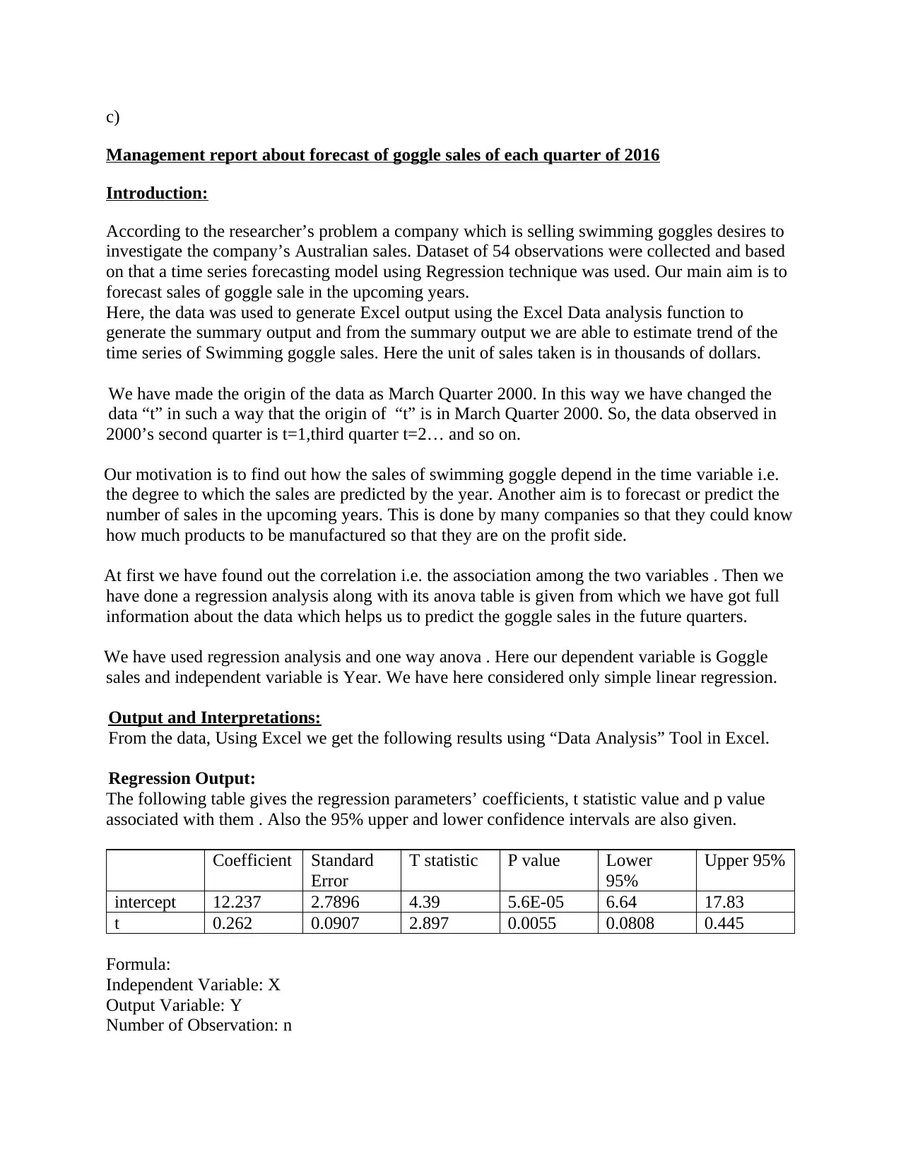
The following table gives the regression parameters’ coefficients, t statistic value and p value
associated with them . Also the 95% upper and lower confidence intervals are also given.
Coefficient Standard
Error
T statistic P value Lower
95%
Upper 95%
intercept 12.237 2.7896 4.39 5.6E-05 6.64 17.83
t 0.262 0.0907 2.897 0.0055 0.0808 0.445
Formula:
Independent Variable: X
Output Variable: Y
Number of Observation: n

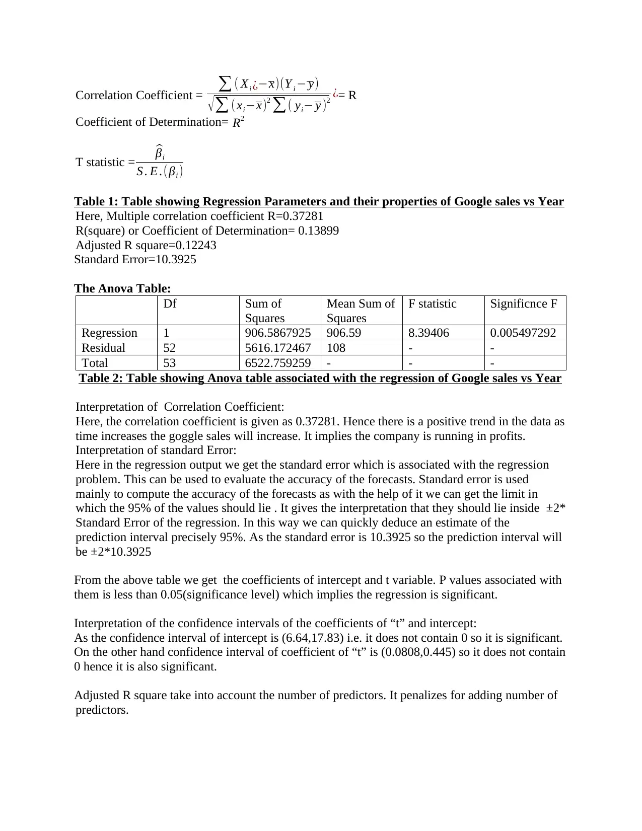
Correlation Coefficient = ∑ ( Xi ¿−x)(Y i − y)
√∑ ( xi−x)2
∑( yi− y )2 ¿= R
Coefficient of Determination= R2
T statistic =
^βi
S . E .(βi )
Table 1: Table showing Regression Parameters and their properties of Google sales vs Year
Here, Multiple correlation coefficient R=0.37281
R(square) or Coefficient of Determination= 0.13899
Adjusted R square=0.12243
Standard Error=10.3925
The Anova Table:
Df Sum of
Squares
Mean Sum of
Squares
F statistic Significnce F
Regression 1 906.5867925 906.59 8.39406 0.005497292
Residual 52 5616.172467 108 - -
Total 53 6522.759259 - - -
Table 2: Table showing Anova table associated with the regression of Google sales vs Year
Interpretation of Correlation Coefficient:
Here, the correlation coefficient is given as 0.37281. Hence there is a positive trend in the data as
time increases the goggle sales will increase. It implies the company is running in profits.
Interpretation of standard Error:
Here in the regression output we get the standard error which is associated with the regression
problem. This can be used to evaluate the accuracy of the forecasts. Standard error is used
mainly to compute the accuracy of the forecasts as with the help of it we can get the limit in
which the 95% of the values should lie . It gives the interpretation that they should lie inside ±2*
Standard Error of the regression. In this way we can quickly deduce an estimate of the
prediction interval precisely 95%. As the standard error is 10.3925 so the prediction interval will
be ±2*10.3925
From the above table we get the coefficients of intercept and t variable. P values associated with
them is less than 0.05(significance level) which implies the regression is significant.
Interpretation of the confidence intervals of the coefficients of “t” and intercept:
As the confidence interval of intercept is (6.64,17.83) i.e. it does not contain 0 so it is significant.
On the other hand confidence interval of coefficient of “t” is (0.0808,0.445) so it does not contain
0 hence it is also significant.
Adjusted R square take into account the number of predictors. It penalizes for adding number of
predictors.

Regression Equation:
Here after collection of data and analyzing we get the following linear trend equation as,
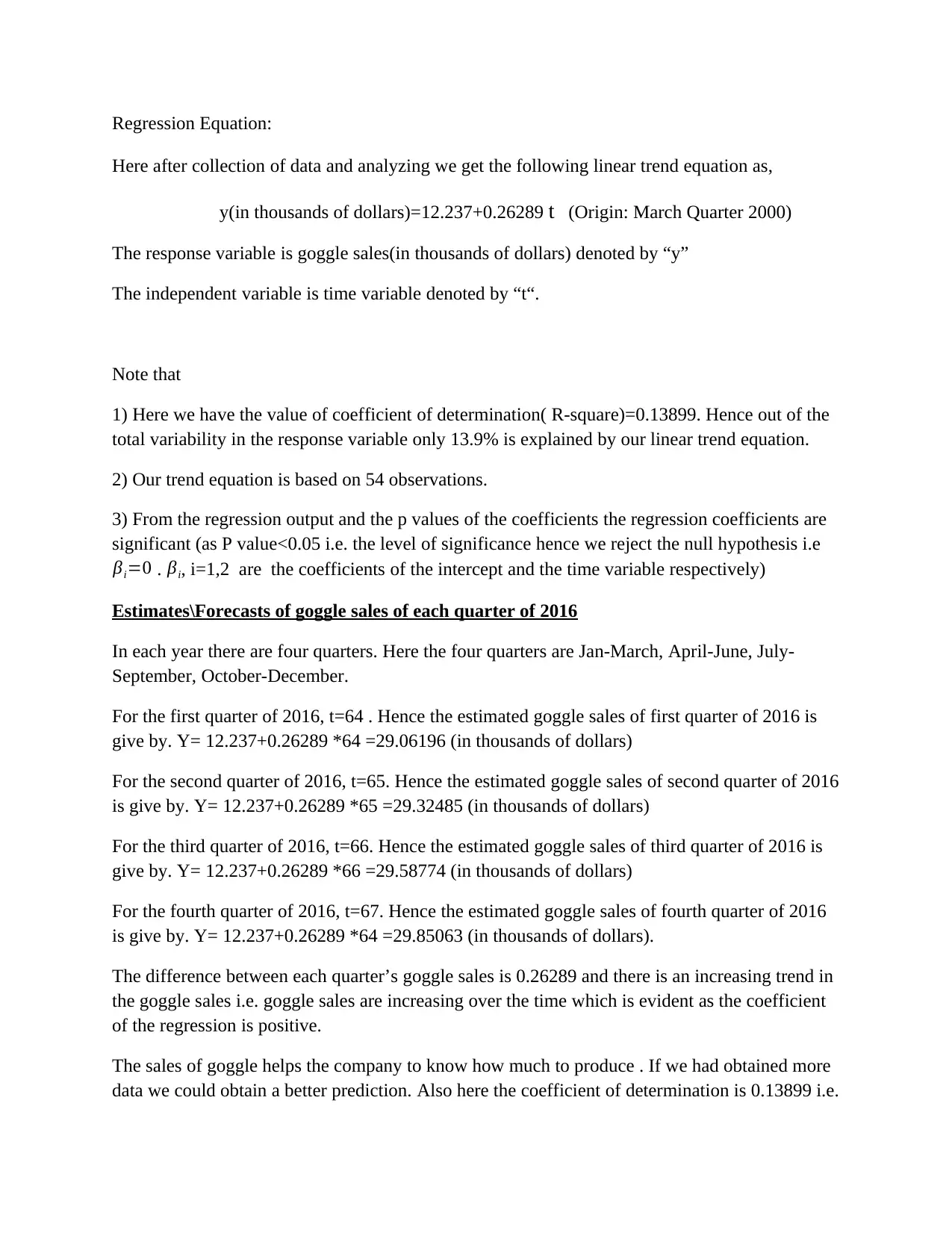
y(in thousands of dollars)=12.237+0.26289 t (Origin: March Quarter 2000)
The response variable is goggle sales(in thousands of dollars) denoted by “y”
The independent variable is time variable denoted by “t“.
Note that
1) Here we have the value of coefficient of determination( R-square)=0.13899. Hence out of the
total variability in the response variable only 13.9% is explained by our linear trend equation.
2) Our trend equation is based on 54 observations.
3) From the regression output and the p values of the coefficients the regression coefficients are
significant (as P value<0.05 i.e. the level of significance hence we reject the null hypothesis i.e
βi=0 . βi, i=1,2 are the coefficients of the intercept and the time variable respectively)
Estimates\Forecasts of goggle sales of each quarter of 2016
In each year there are four quarters. Here the four quarters are Jan-March, April-June, July-
September, October-December.
For the first quarter of 2016, t=64 . Hence the estimated goggle sales of first quarter of 2016 is
give by. Y= 12.237+0.26289 *64 =29.06196 (in thousands of dollars)
For the second quarter of 2016, t=65. Hence the estimated goggle sales of second quarter of 2016
is give by. Y= 12.237+0.26289 *65 =29.32485 (in thousands of dollars)
For the third quarter of 2016, t=66. Hence the estimated goggle sales of third quarter of 2016 is
give by. Y= 12.237+0.26289 *66 =29.58774 (in thousands of dollars)
For the fourth quarter of 2016, t=67. Hence the estimated goggle sales of fourth quarter of 2016
is give by. Y= 12.237+0.26289 *64 =29.85063 (in thousands of dollars).
The difference between each quarter’s goggle sales is 0.26289 and there is an increasing trend in
the goggle sales i.e. goggle sales are increasing over the time which is evident as the coefficient
of the regression is positive.
The sales of goggle helps the company to know how much to produce . If we had obtained more
data we could obtain a better prediction. Also here the coefficient of determination is 0.13899 i.e.

only 14% of the total variation of the sales is explained by the time variable. Hence we should
check higher degree of regression i.e. we should check whether the data follows a quadratic trend
or cubic trend . We could have an idea of the trend it is following by a scatterplot . But above all
we should take more values into consideration so that our output result is better.
References:
Sheldon, Ross (2010). Introductory Statistics, Academic Press,USA.
Hoel,P.G.,(1971),Introduction to Mathematical Statistics,Fourth Edition,USA
Feller,William(2013),An introduction to Probability Theory and Its Applications,Volume I,Third
Edition,U.K.
Du Prel, J.-B., Hommel, G., Röhrig, B., & Blettner, M. (2009). Confidence Interval or P-Value?:
Part 4 of a Series on Evaluation of Scientific Publications. Deutsches Ärzteblatt
International, 106(19), 335–339.
Akobeng AK. Confidence intervals and p-values in clinical decision making. Acta Paediatr.
2008;97:1004–1007
Altman D, Bland JM. Confidence intervals illuminate absence of evidence. BMJ.
2004;328:1016–1017
Question 3
(i)
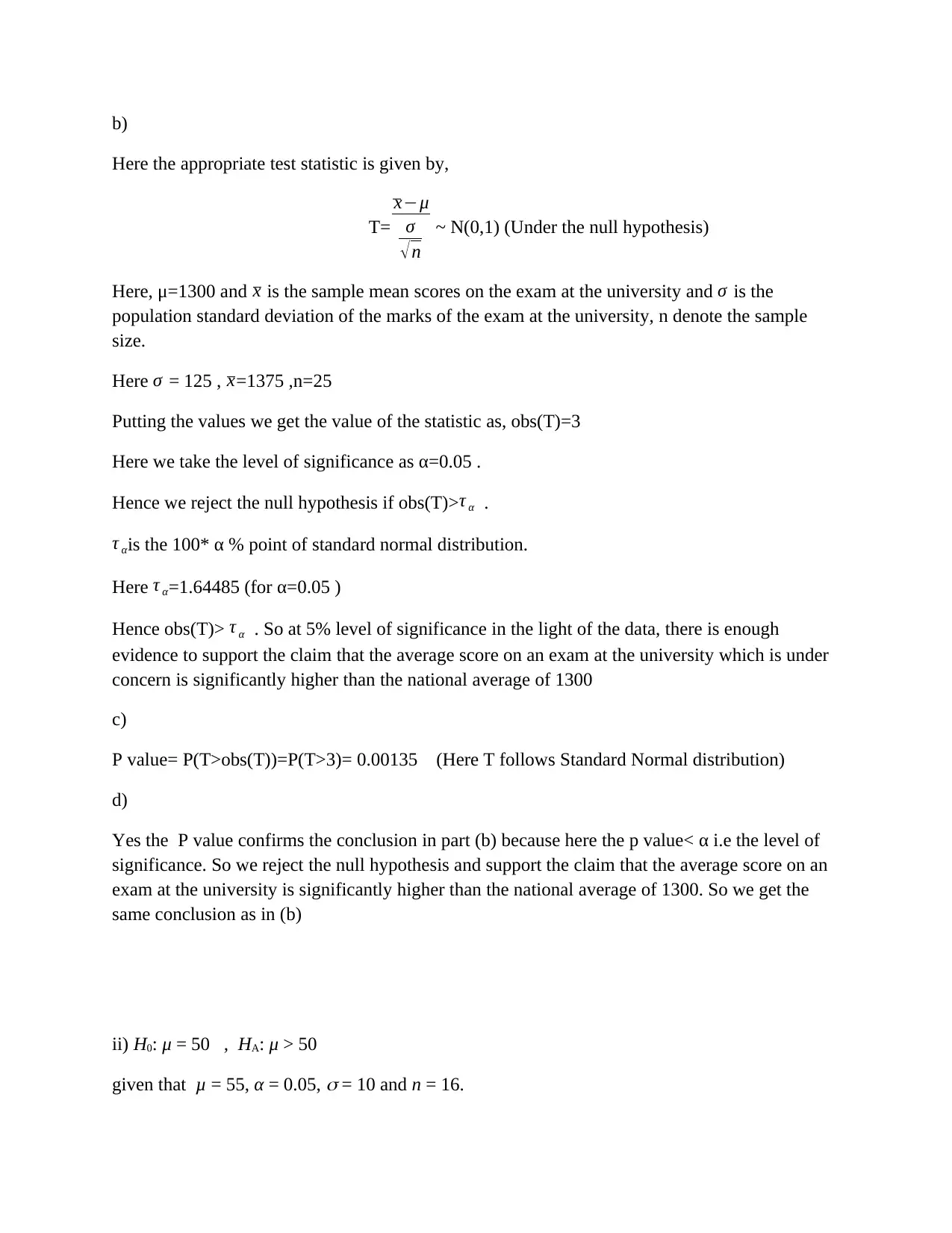
a) According to the problem the suitable null and alternative hypotheses are given as below, H0
:μ=1300 H1: μ>1300 (μ is denoted as the population mean of the exam at the university)

b)
Here the appropriate test statistic is given by,
T=
x−μ
σ
√ n
~ N(0,1) (Under the null hypothesis)
Here, μ=1300 and x is the sample mean scores on the exam at the university and σ is the
population standard deviation of the marks of the exam at the university, n denote the sample
size.
Here σ = 125 , x=1375 ,n=25
Putting the values we get the value of the statistic as, obs(T)=3
Here we take the level of significance as α=0.05 .
Hence we reject the null hypothesis if obs(T)>τ α .
τ αis the 100* α % point of standard normal distribution.
Here τ α=1.64485 (for α=0.05 )
Hence obs(T)> τ α . So at 5% level of significance in the light of the data, there is enough
evidence to support the claim that the average score on an exam at the university which is under
concern is significantly higher than the national average of 1300
c)
P value= P(T>obs(T))=P(T>3)= 0.00135 (Here T follows Standard Normal distribution)
d)
Yes the P value confirms the conclusion in part (b) because here the p value< α i.e the level of
significance. So we reject the null hypothesis and support the claim that the average score on an
exam at the university is significantly higher than the national average of 1300. So we get the
same conclusion as in (b)
ii) H0: μ = 50 , HA: μ > 50
given that μ = 55, α = 0.05,
 = 10 and n = 16.

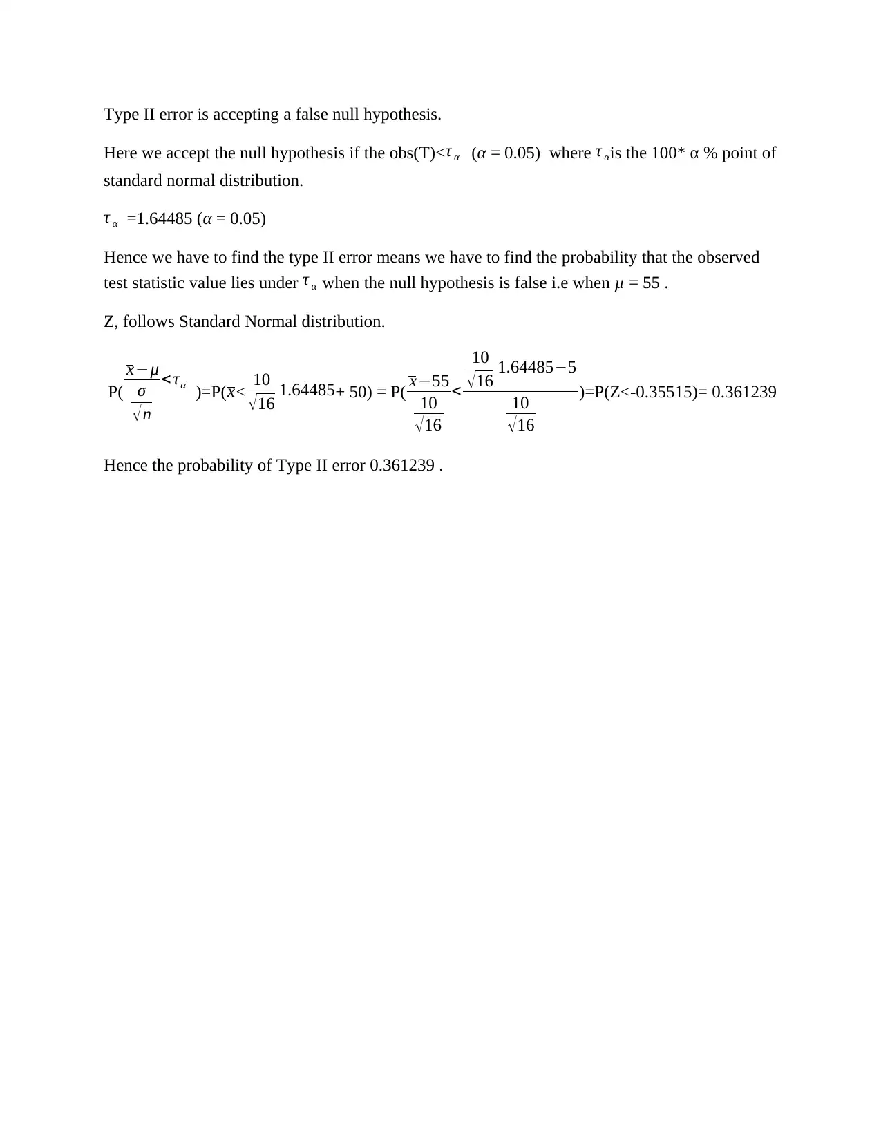
Type II error is accepting a false null hypothesis.
Here we accept the null hypothesis if the obs(T)< τ α (α = 0.05) where τ αis the 100* α % point of
standard normal distribution.
τ α =1.64485 (α = 0.05)
Hence we have to find the type II error means we have to find the probability that the observed
test statistic value lies under τ α when the null hypothesis is false i.e when μ = 55 .
Z, follows Standard Normal distribution.
P(
x−μ
σ
√ n
< τα )=P(x< 10
√16 1.64485+ 50) = P( x−55
10
√ 16
<
10
√ 16 1.64485−5
10
√ 16
)=P(Z<-0.35515)= 0.361239
Hence the probability of Type II error 0.361239 .