STAT 193: Statistics in Practice Project Assignment

This project assignment for STAT 193 Statistics in Practice covers topics such as dataset, weekly income, marital status and ethnicity, highest qualification and income. It includes insights on hypothesis testing, ANOVA test, and more. The assignment also mentions the subject, course code, and college/university.

STAT 193 Statistics in Practice
Project Assignment
Question 1: The dataset
o Gender is a nominal, categorical variable. Because there is no natural order, only
categorized in Male or Female.
o Age is a continuous, numerical variable. The minimum value is 15 years and the
maximum value is 45 years.
o Ethnicity is a nominal, categorical variable. The possible values the variable takes are
European, Pacific, Maori, or Other.
o Marital is a nominal, categorical variable. The possible values the variable takes are
Married, Never, Previously or Other.
o Qualification is a nominal, categorical variable. The possible values the variable takes
are Degree, School, Vocational or None.
o PostSchool is a nominal, categorical variable. Because there is no natural order, only
categorized in Yes or No.
o Hours is a continuous, numerical variable. The minimum value is 2 and the maximum
value is 70 years.
o Income is a discrete, numerical variable. The minimum value is 11 and the maximum
value is 1789.
Question 2: Weekly Income
(a) Histogram:
1

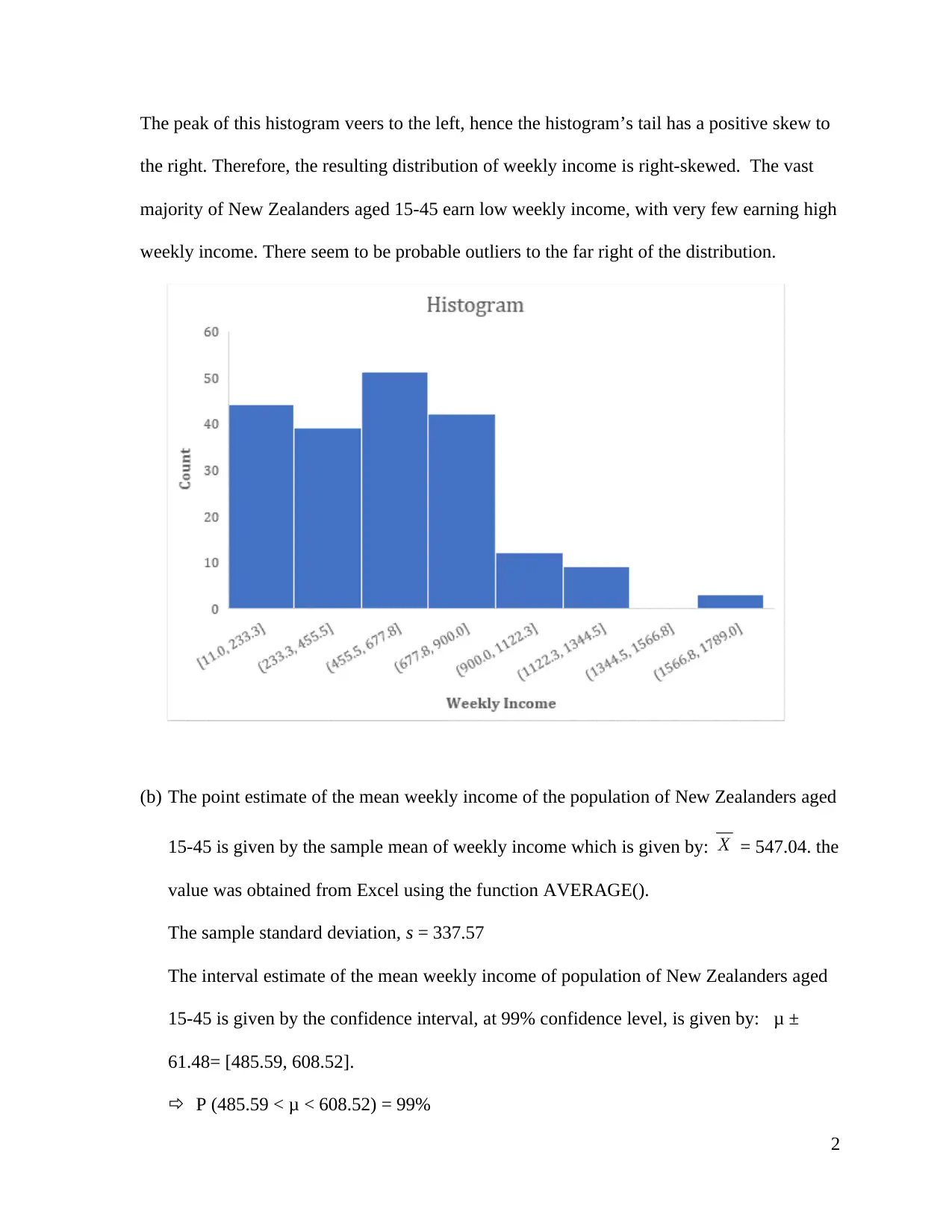
The peak of this histogram veers to the left, hence the histogram’s tail has a positive skew to
the right. Therefore, the resulting distribution of weekly income is right-skewed. The vast
majority of New Zealanders aged 15-45 earn low weekly income, with very few earning high
weekly income. There seem to be probable outliers to the far right of the distribution.
(b) The point estimate of the mean weekly income of the population of New Zealanders aged
15-45 is given by the sample mean of weekly income which is given by: = 547.04. the
value was obtained from Excel using the function AVERAGE().
The sample standard deviation, s = 337.57
The interval estimate of the mean weekly income of population of New Zealanders aged
15-45 is given by the confidence interval, at 99% confidence level, is given by: μ ±
61.48= [485.59, 608.52].
 P (485.59 < μ < 608.52) = 99%
2

Since, the sample size is greater than 30, the distribution of the random variable was
approximated with a normal distribution. In Excel, we used the function,
CONFIDENCE.NORM(alpha, standard deviation, sample size)
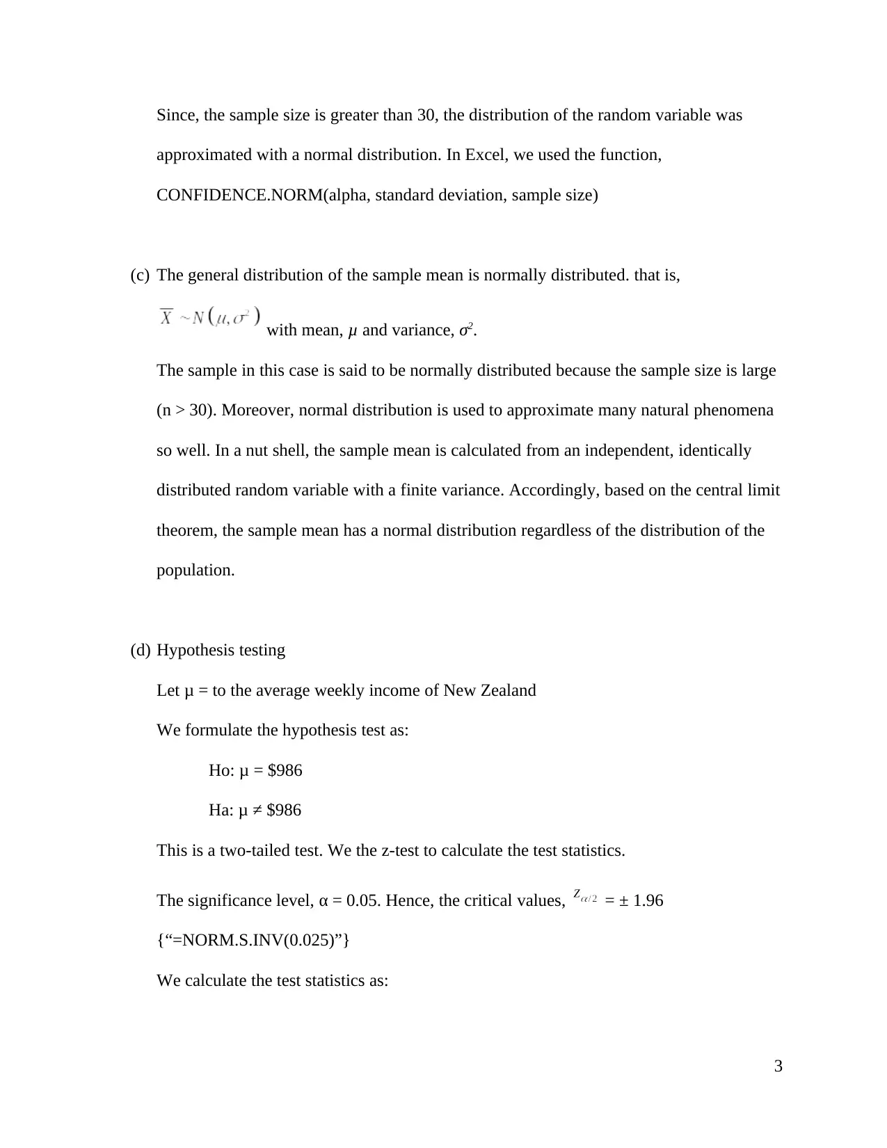
(c) The general distribution of the sample mean is normally distributed. that is,
with mean, μ and variance, σ2.
The sample in this case is said to be normally distributed because the sample size is large
(n > 30). Moreover, normal distribution is used to approximate many natural phenomena
so well. In a nut shell, the sample mean is calculated from an independent, identically
distributed random variable with a finite variance. Accordingly, based on the central limit
theorem, the sample mean has a normal distribution regardless of the distribution of the
population.
(d) Hypothesis testing
Let μ = to the average weekly income of New Zealand
We formulate the hypothesis test as:
Ho: μ = $986
Ha: μ ≠ $986
This is a two-tailed test. We the z-test to calculate the test statistics.
The significance level, α = 0.05. Hence, the critical values, = ± 1.96
{“=NORM.S.INV(0.025)”}
We calculate the test statistics as:
3

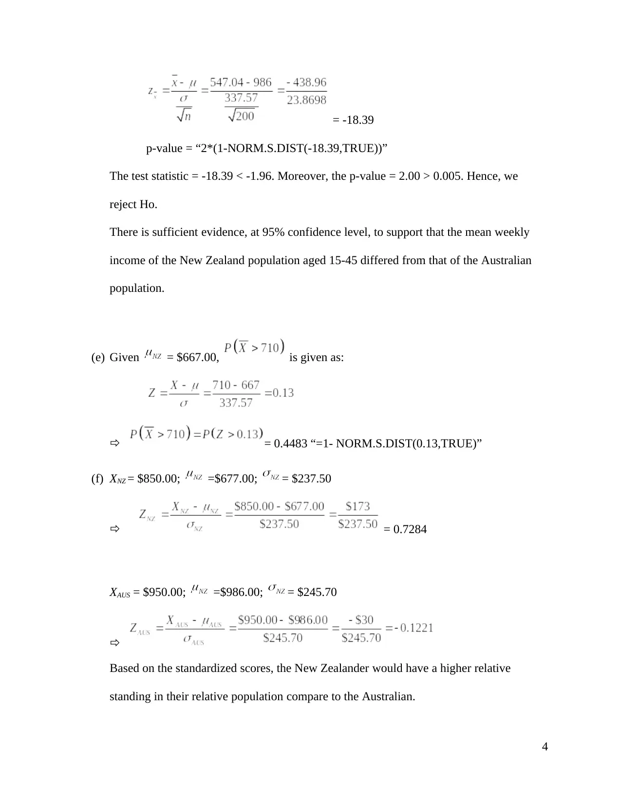
= -18.39
p-value = “2*(1-NORM.S.DIST(-18.39,TRUE))”
The test statistic = -18.39 < -1.96. Moreover, the p-value = 2.00 > 0.005. Hence, we
reject Ho.
There is sufficient evidence, at 95% confidence level, to support that the mean weekly
income of the New Zealand population aged 15-45 differed from that of the Australian
population.
(e) Given = $667.00, is given as:
 = 0.4483 “=1- NORM.S.DIST(0.13,TRUE)”
(f) XNZ = $850.00; =$677.00; = $237.50
 = 0.7284
XAUS = $950.00; =$986.00; = $245.70

Based on the standardized scores, the New Zealander would have a higher relative
standing in their relative population compare to the Australian.
4

Question 3: Marital Status and ethnicity
(a) The graph suggests that there is an association between Marital and Ethnicity. We can
see from the graph that the number of individuals with a certain marital status vary with
their ethnicity. For instance, there are more Pacific citizens are married than Maori.
Similarly, less Pacific citizens have never married compared to the Maori.
(b) Null Hypothesis, Ho: Marital status is not associated with Ethnicity
Alternative hypothesis, Ha: Marital status is associated with Ethnicity.
(c) The number of Pacific people who are married = 0
Total married = 64
(d) i. Percentage of people who have never married that are Maori = 16/90 = 17.78%
ii. Percentage of Maori people who have ever married = 16/21 = 76.19%
(e) Test statistic value = χ2 = 21.69
Degrees of freedom = 9
p-value = 0.0099 = 0.01
At level of significance, α = 0.005, the p-value is < 0.05, the null hypothesis is rejected.
There is sufficient evidence to support the conclusion that marital status is associated
with ethnicity. In other words, the marital status of people changes with their ethnicity.
5

(f) The conclusion ins part (e) was not surprising given it was similar with my answer in part
(a). moreover, examine the pattern of number in the chart, it was noted that more Maori
people were never married than pacific people. The number of the other marital status
differed among the ethnicity groups. Therefore, as the conclusion indicated, the variable
Marital changes with the variable Ethnicity.
Question 4: Highest Qualification and Income
(a) The side-by-side boxplots of Income by Qualification suggest that the mean weekly
income differs among qualification levels. The location of the boxplot for each
qualification level is different, which indicates that the median of weekly income is
different for each qualification level. For instance, the median weekly income for people
with a degree is higher than the weekly income for people without any qualification.
Similarly, the median weekly income for “None” qualification is higher than the median
weekly income of people with “school” qualification.
(b) Null hypothesis, Ho: μ1 = μ2 = μ3 = μ4 (the mean weekly income is equal for all
qualification levels)
Alternative hypothesis, Ha: μ1 ≠ μ2 ≠ μ3 ≠ μ4 (the mean weekly income is not equal for all
qualification level, at least one is different)
(c) The results of the ANOVA test are such that:
The test statistic = F = 42.051
Degrees of freedom = 3, and 196; total = 199
6

p-value = 0.0000002 < 0.001
At 5% level of significance, we reject the null hypothesis, Ho, given that the p-value ≈
0.0000 < 0.05. There is sufficient statistical evidence to conclude that the mean weekly income is
not equal for all qualification levels.
(d) Calculating the degree of freedom was done as follows:
Qualification levels = 4 = m => df (Factor) = m – 1 = 4 -1 = 3
Sample size = n = 200 => df (Error) = n – m = 200 – 4 = 196
 df (Total) = n – 1 = 200 – 1 = 199 = (m - 1) + (n - m) = 3 + 196 = 199
(e) The results indicate that there is sufficient evidence of a difference in mean income at 5%
significance level for the following pairs:
- Degree & None
- Degree & School
- None & Vocational
This is because the p-values for the difference in mean income between qualification
groups was reported to be 0.0000 which is less than the level of significance (< 0.05).
Therefore, we conclude that there is significant difference in mean income between these
pairs. On the other hand, the p-value for the pair, None & School was obtained as 0.85 >
0.05, we reject Ho, and conclude that there is no significant difference in mean income
between this pair.
(f) For the ANOVA test to be valid, the following assumptions must be met:
7

- The population from which each group is drawn is normally distributed
- There is a common variance for all populations
- The samples are independently drawn from each other, and the observations
from this samples are randomly selected
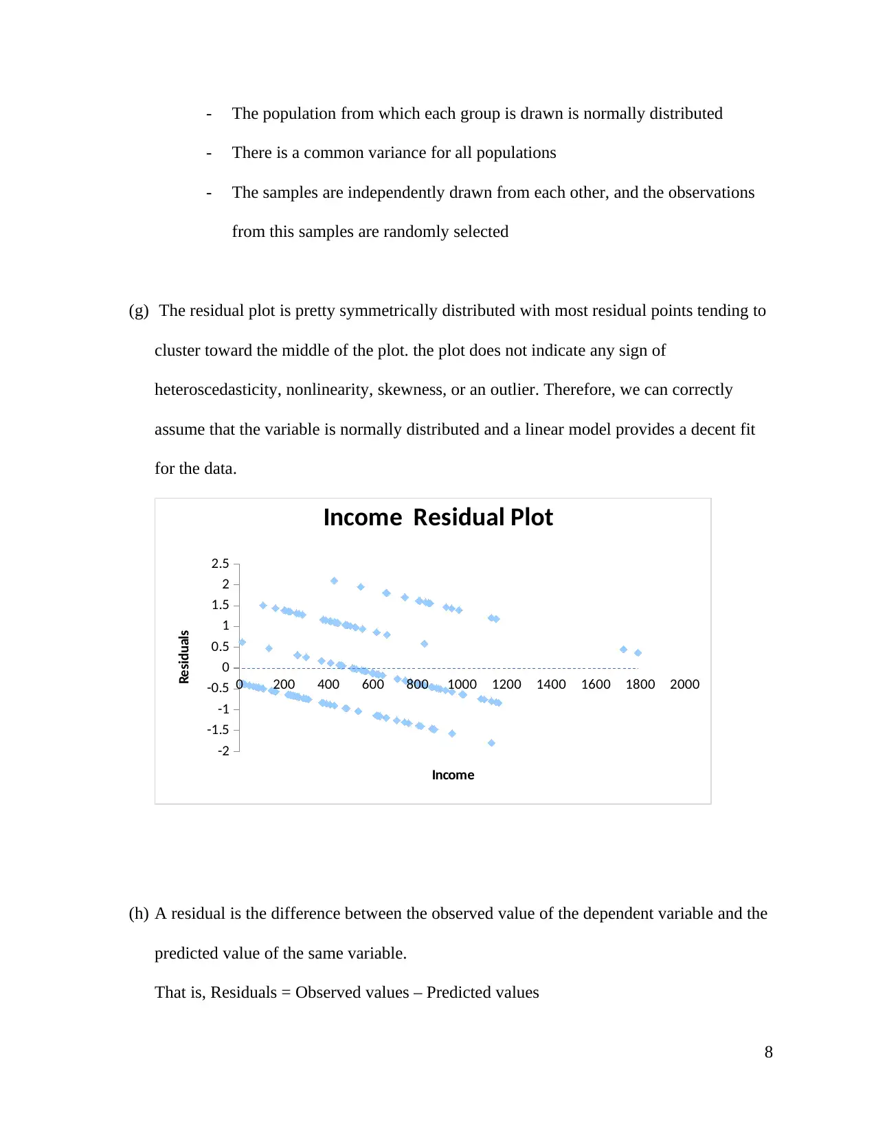
(g) The residual plot is pretty symmetrically distributed with most residual points tending to
cluster toward the middle of the plot. the plot does not indicate any sign of
heteroscedasticity, nonlinearity, skewness, or an outlier. Therefore, we can correctly
assume that the variable is normally distributed and a linear model provides a decent fit
for the data.
0 200 400 600 800 1000 1200 1400 1600 1800 2000
-2
-1.5
-1
-0.5
0
0.5
1
1.5
2
2.5
Income Residual Plot
Income
Residuals
(h) A residual is the difference between the observed value of the dependent variable and the
predicted value of the same variable.
That is, Residuals = Observed values – Predicted values
8