STAT 381 – Summer 2019
VerifiedAdded on 2022/11/23
|8
|624
|54
AI Summary
Get answers to your STAT 381 – Summer 2019 assignments, essays, dissertation and study material by our experts. Learn from our vast document library with solved assignments, essays, dissertation and study material for your courses.
Contribute Materials
Your contribution can guide someone’s learning journey. Share your
documents today.

STAT 381 – Summer 2019
1
1
Secure Best Marks with AI Grader
Need help grading? Try our AI Grader for instant feedback on your assignments.
Answer 1
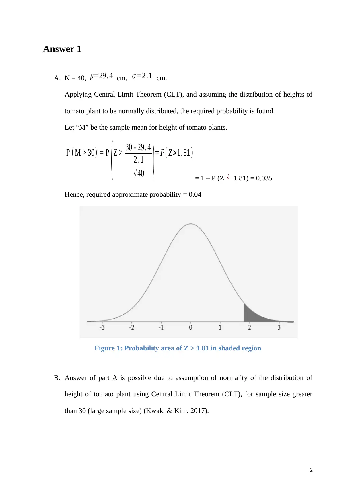
A. N = 40, μ=29 . 4 cm, σ =2 .1 cm.
Applying Central Limit Theorem (CLT), and assuming the distribution of heights of
tomato plant to be normally distributed, the required probability is found.
Let “M” be the sample mean for height of tomato plants.
P ( M > 30) = P
( Z > 30 - 29 . 4
2 . 1
√ 40 )=P( Z >1. 81 )
= 1 – P (Z ¿ 1.81) = 0.035
Hence, required approximate probability = 0.04
Figure 1: Probability area of Z > 1.81 in shaded region
B. Answer of part A is possible due to assumption of normality of the distribution of
height of tomato plant using Central Limit Theorem (CLT), for sample size greater
than 30 (large sample size) (Kwak, & Kim, 2017).
2
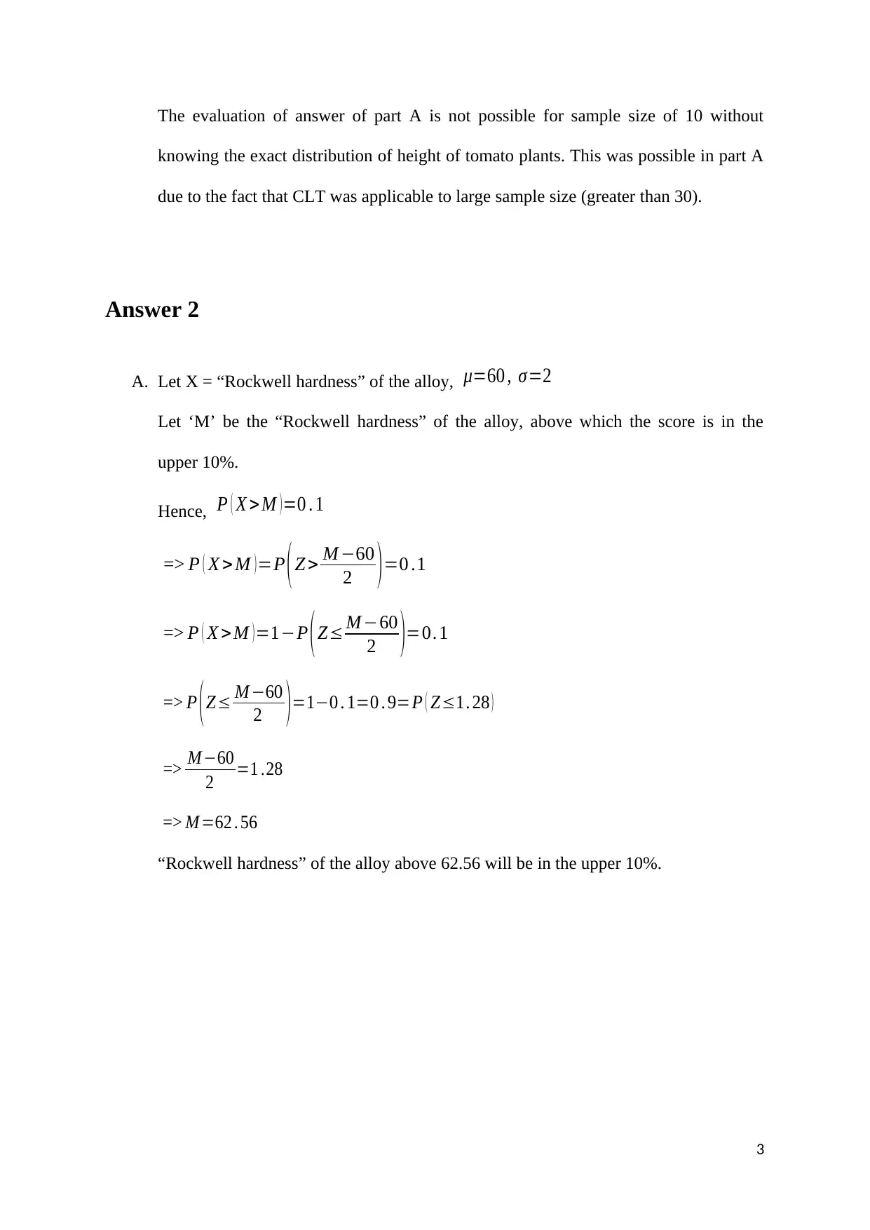
The evaluation of answer of part A is not possible for sample size of 10 without
knowing the exact distribution of height of tomato plants. This was possible in part A
due to the fact that CLT was applicable to large sample size (greater than 30).
Answer 2
A. Let X = “Rockwell hardness” of the alloy, μ=60 , σ=2
Let ‘M’ be the “Rockwell hardness” of the alloy, above which the score is in the
upper 10%.
Hence, P ( X > M ) =0 . 1
=> P ( X > M ) =P ( Z > M −60
2 ) =0 .1
=> P ( X >M ) =1−P ( Z≤ M −60
2 )=0. 1
=> P ( Z≤ M −60
2 ) =1−0 . 1=0 . 9=P ( Z≤1. 28 )
=> M −60
2 =1 .28
=> M =62 . 56
“Rockwell hardness” of the alloy above 62.56 will be in the upper 10%.
3
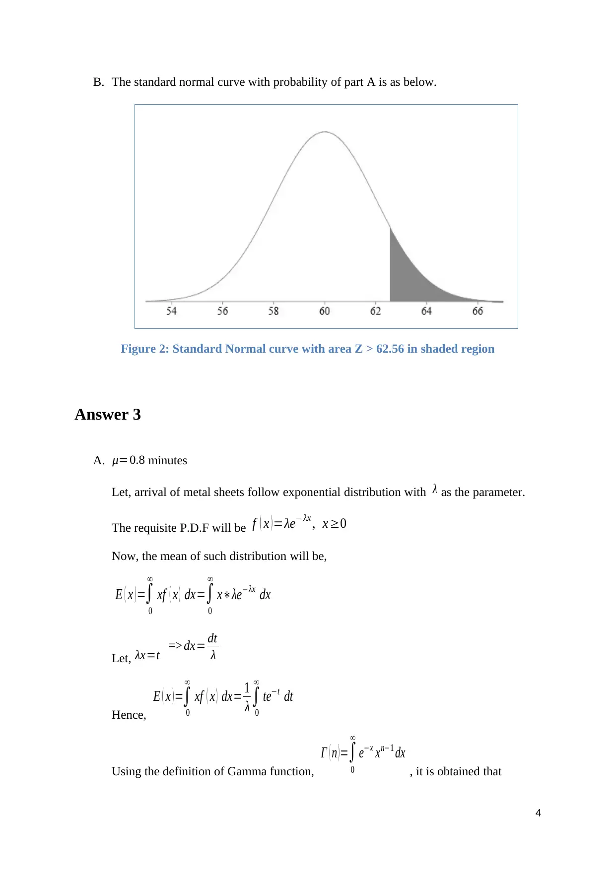
B. The standard normal curve with probability of part A is as below.
Figure 2: Standard Normal curve with area Z > 62.56 in shaded region
Answer 3
A. μ=0.8 minutes
Let, arrival of metal sheets follow exponential distribution with λ as the parameter.
The requisite P.D.F will be f ( x ) =λe− λx , x ≥0
Now, the mean of such distribution will be,
E ( x ) =∫
0
∞
xf ( x ) dx=∫
0
∞
x∗λe−λx dx
Let, λx=t => dx= dt
λ
Hence,
E ( x ) =∫
0
∞
xf ( x ) dx= 1
λ ∫
0
∞
te−t dt
Using the definition of Gamma function,
Γ ( n ) =∫
0
∞
e−x xn−1 dx
, it is obtained that
4
Secure Best Marks with AI Grader
Need help grading? Try our AI Grader for instant feedback on your assignments.
E ( x ) =∫
0
∞
xf ( x ) dx= 1
λ ∫
0
∞
te−t dt = 1
λ Γ ( 2 ) = 1
λ as Γ ( 2 ) = ( 2−1 ) !=1
So,
1
λ =0 . 8=> λ= 1
0 .8 =1. 25
B. Probability of more than 2 minutes wait time between arrivals is evaluated as
P ( X >2 ) =∫
2
∞
1 .25∗e−1. 25 x dx= lim
X−¿ ∞
∫
2
X
1 .25∗e−1. 25 x dx
P ( X >2 ) = lim
X −¿ ∞
∫
2
X
1. 25∗e−1 . 25 x dx=1 . 25∗ lim
X −¿ ∞ [ e−1 .25 x
−1. 25 ]2
X
=− lim
X−¿∞ [ e−1. 25 X −e−2. 5
1 ]= 1
e2. 5
So,
P ( X >2 ) = 1
e2. 5 =0 . 08
(Krishnamoorthy, 2016)
Required probability for wait time of more than 2 minutes is 0.08.
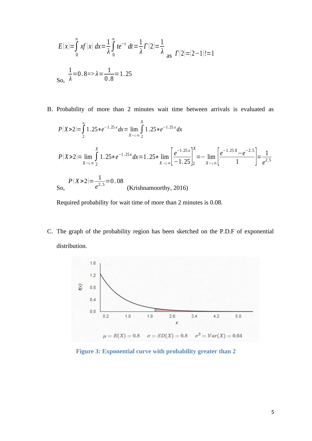
C. The graph of the probability region has been sketched on the P.D.F of exponential
distribution.
Figure 3: Exponential curve with probability greater than 2
5
0
∞
xf ( x ) dx= 1
λ ∫
0
∞
te−t dt = 1
λ Γ ( 2 ) = 1
λ as Γ ( 2 ) = ( 2−1 ) !=1
So,
1
λ =0 . 8=> λ= 1
0 .8 =1. 25
B. Probability of more than 2 minutes wait time between arrivals is evaluated as
P ( X >2 ) =∫
2
∞
1 .25∗e−1. 25 x dx= lim
X−¿ ∞
∫
2
X
1 .25∗e−1. 25 x dx
P ( X >2 ) = lim
X −¿ ∞
∫
2
X
1. 25∗e−1 . 25 x dx=1 . 25∗ lim
X −¿ ∞ [ e−1 .25 x
−1. 25 ]2
X
=− lim
X−¿∞ [ e−1. 25 X −e−2. 5
1 ]= 1
e2. 5
So,
P ( X >2 ) = 1
e2. 5 =0 . 08
(Krishnamoorthy, 2016)
Required probability for wait time of more than 2 minutes is 0.08.
C. The graph of the probability region has been sketched on the P.D.F of exponential
distribution.
Figure 3: Exponential curve with probability greater than 2
5
Answer 4
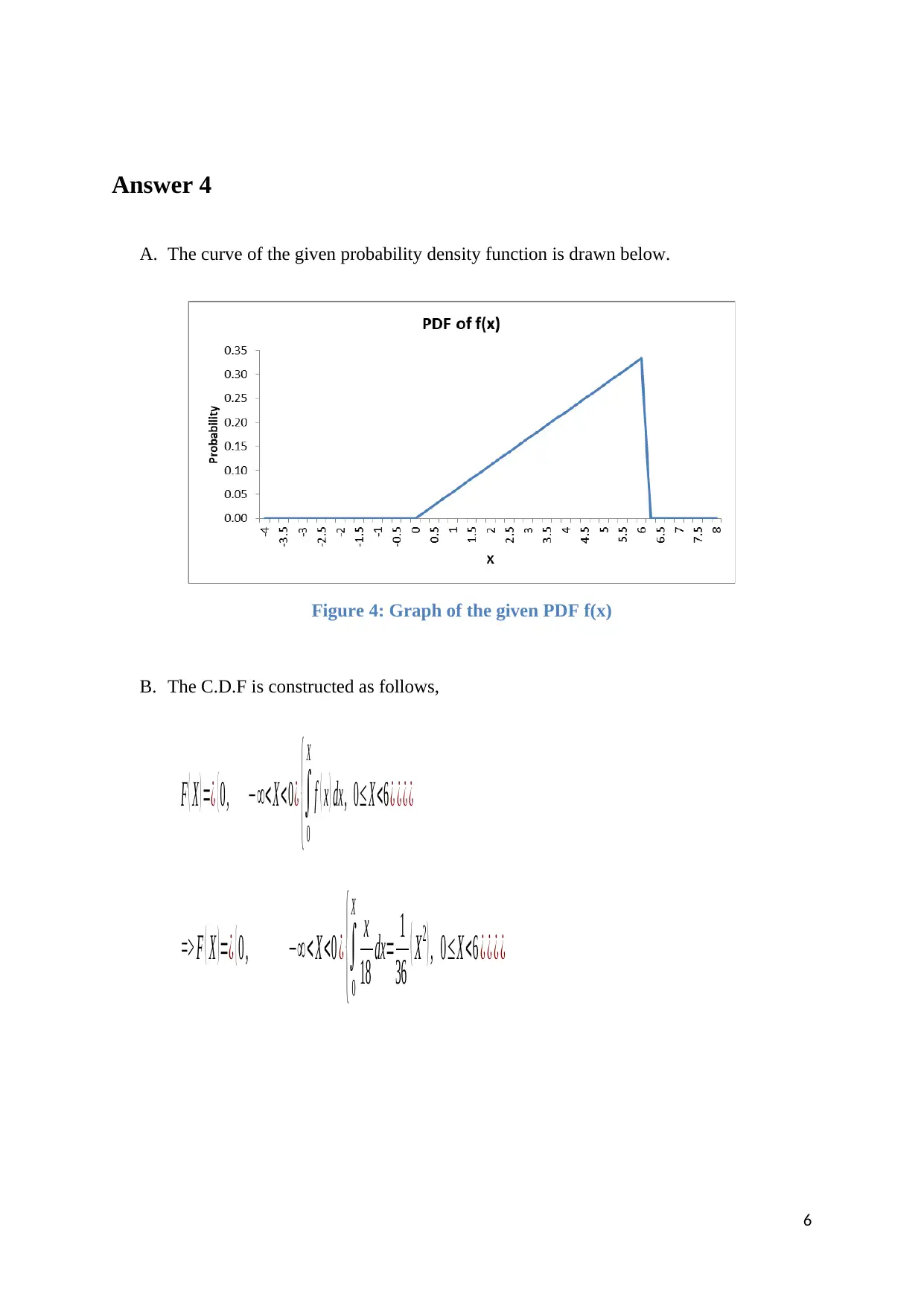
A. The curve of the given probability density function is drawn below.
Figure 4: Graph of the given PDF f(x)
B. The C.D.F is constructed as follows,
F ( X ) =¿ { 0 , −∞< X < 0 ¿ {∫
0
X
f ( x ) dx , 0≤ X <6 ¿ ¿ ¿ ¿
=> F ( X ) =¿ { 0 , −∞< X <0 ¿ {∫
0
X x
18 dx= 1
36 ( X2 ) , 0≤X <6 ¿ ¿ ¿ ¿
6
A. The curve of the given probability density function is drawn below.
Figure 4: Graph of the given PDF f(x)
B. The C.D.F is constructed as follows,
F ( X ) =¿ { 0 , −∞< X < 0 ¿ {∫
0
X
f ( x ) dx , 0≤ X <6 ¿ ¿ ¿ ¿
=> F ( X ) =¿ { 0 , −∞< X <0 ¿ {∫
0
X x
18 dx= 1
36 ( X2 ) , 0≤X <6 ¿ ¿ ¿ ¿
6
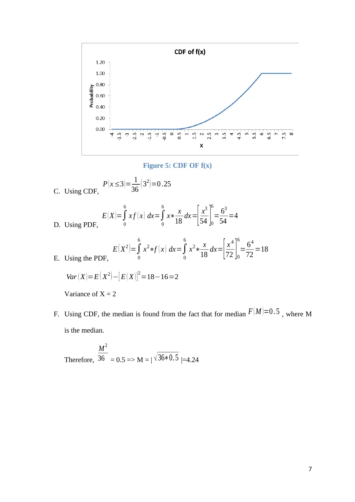
Figure 5: CDF OF f(x)
C. Using CDF,
P ( x ≤3 ) = 1
36 ( 32 ) =0 .25
D. Using PDF,
E ( X ) =∫
0
6
x f ( x ) dx=∫
0
6
x∗ x
18 dx =[ x3
54 ]0
6
= 63
54 =4
E. Using the PDF,
E ( X2 ) =∫
0
6
x2∗f ( x ) dx=∫
0
6
x2∗ x
18 dx= [ x 4
72 ] 0
6
= 64
72 =18
Var ( X ) =E ( X2 ) − [ E ( X ) ] 2=18−16=2
Variance of X = 2
F. Using CDF, the median is found from the fact that for median F ( M ) =0 . 5 , where M
is the median.
Therefore,
M 2
36 = 0.5 => M = | √ 36∗0. 5 |=4.24
7
Paraphrase This Document
Need a fresh take? Get an instant paraphrase of this document with our AI Paraphraser
Answer 5
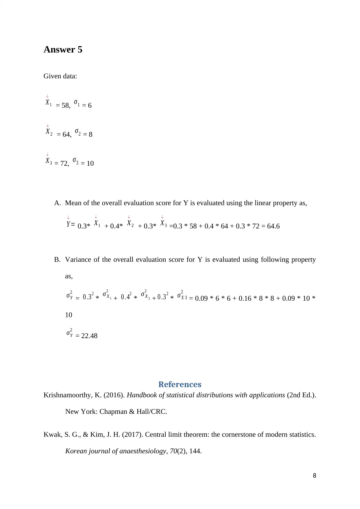
Given data:
X
¿
1 = 58, σ1 = 6
X
¿
2 = 64, σ2 = 8
X
¿
3 = 72, σ3 = 10
A. Mean of the overall evaluation score for Y is evaluated using the linear property as,
Y
¿
= 0.3* X
¿
1 + 0.4* X
¿
2 + 0.3* X
¿
3 =0.3 * 58 + 0.4 * 64 + 0.3 * 72 = 64.6
B. Variance of the overall evaluation score for Y is evaluated using following property
as,
σY
2
= 0 .32
* σ X 1
2
+ 0 . 42
* σ X 2
2
+ 0 .32
* σ X 3
2
= 0.09 * 6 * 6 + 0.16 * 8 * 8 + 0.09 * 10 *
10
σY
2
= 22.48
References
Krishnamoorthy, K. (2016). Handbook of statistical distributions with applications (2nd Ed.).
New York: Chapman & Hall/CRC.
Kwak, S. G., & Kim, J. H. (2017). Central limit theorem: the cornerstone of modern statistics.
Korean journal of anaesthesiology, 70(2), 144.
8
1 out of 8
Your All-in-One AI-Powered Toolkit for Academic Success.
+13062052269
info@desklib.com
Available 24*7 on WhatsApp / Email
![[object Object]](/_next/static/media/star-bottom.7253800d.svg)
Unlock your academic potential
© 2024 | Zucol Services PVT LTD | All rights reserved.