StAT2000-Quantitative Analysis of a sample of 400 US students working in US

b) Probability of exactly two = 0.06 ii) Probability of more than two = P(3) + P(4) +P(5) +P(6) = 0.28 + 0.12 +0.0 + 0.94 = 0.78 iii) Probability of atleast three = P(3) + P(4) +P(5) +P(6) = 0.28 + 0.12 +0.0 + 0.38 = 0.78 f) Probability of success = Probability of person being involved in sales or occupation “2” = 0.06 Hence, probability of failure =

STAT2000-Quantitative Analysis
STUDENT ID:
[Pick the date]

Introduction
A random sample of 400 individuals working in US has been provided and the objective is to
conduct a statistical analysis by selecting a unique set of 50 observations based on the
underlying student ID. There are three tasks that need to be performed which require the use
of both descriptive and inferential statistical techniques. The output obtained along with
interpretation of the same would be provided in this report.
Task 1
The sample of 50 observations has been obtained and listed in Appendix 1.
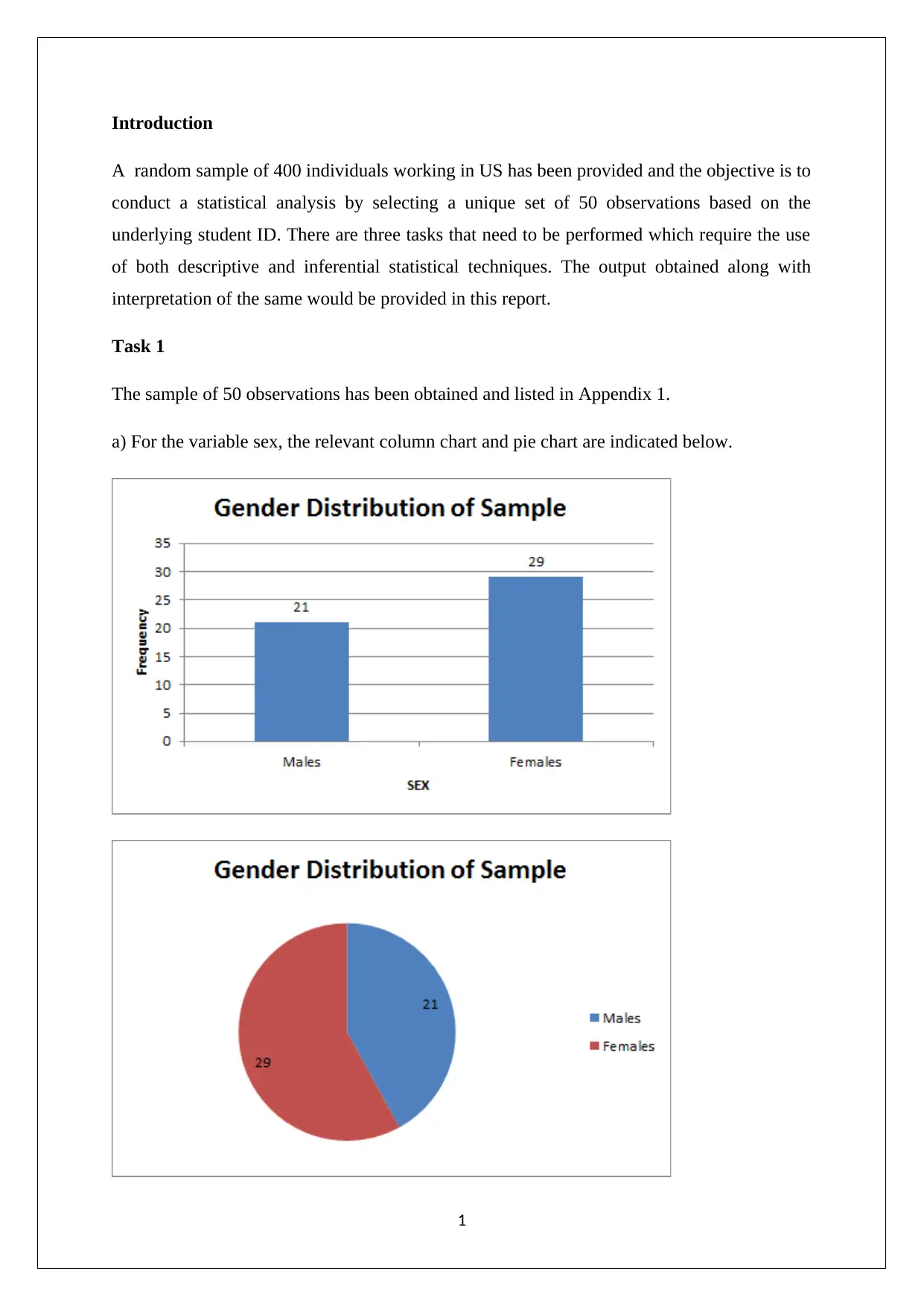
a) For the variable sex, the relevant column chart and pie chart are indicated below.
1

It is apparent from the above graphs and charts that the selected sample of 50 individuals
selected comprises of 21 males and 29 females and hence representation of females is higher
than males which may not be true in the actual population.
Task 2
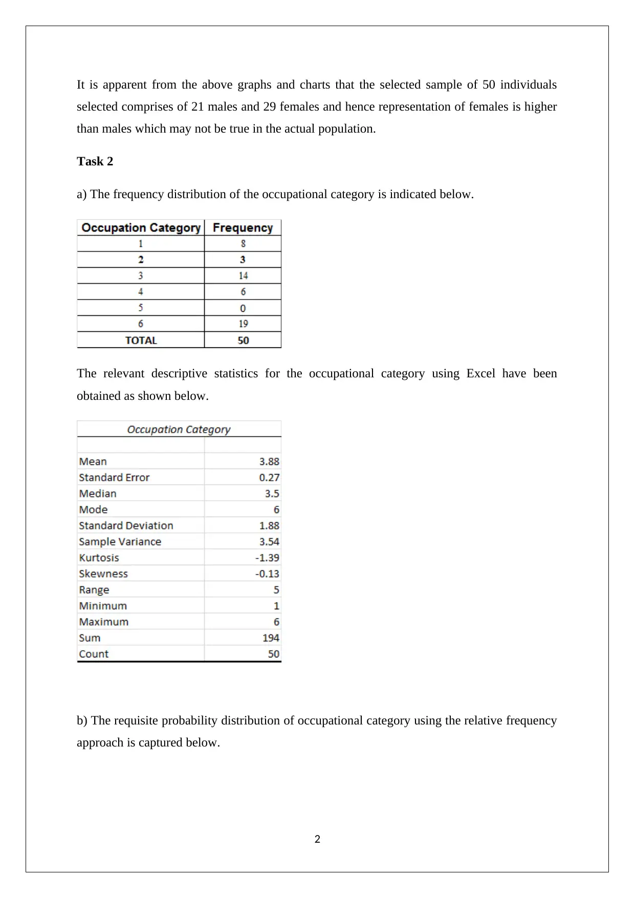
a) The frequency distribution of the occupational category is indicated below.
The relevant descriptive statistics for the occupational category using Excel have been
obtained as shown below.
b) The requisite probability distribution of occupational category using the relative frequency
approach is captured below.
2

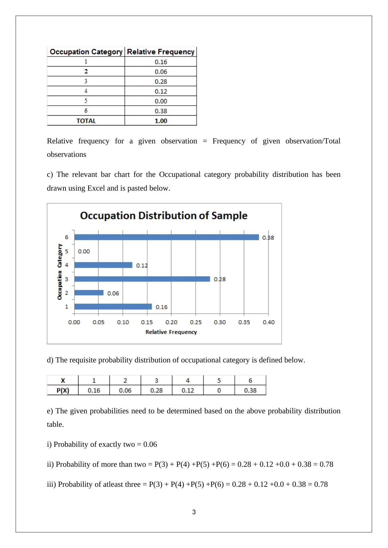
Relative frequency for a given observation = Frequency of given observation/Total
observations
c) The relevant bar chart for the Occupational category probability distribution has been
drawn using Excel and is pasted below.
d) The requisite probability distribution of occupational category is defined below.
e) The given probabilities need to be determined based on the above probability distribution
table.
i) Probability of exactly two = 0.06
ii) Probability of more than two = P(3) + P(4) +P(5) +P(6) = 0.28 + 0.12 +0.0 + 0.38 = 0.78
iii) Probability of atleast three = P(3) + P(4) +P(5) +P(6) = 0.28 + 0.12 +0.0 + 0.38 = 0.78
3

f) Probability of success = Probability of person being involved in sales or occupation “2” =
0.06
Hence, probability of failure = 1-0.06 = 0.94
The binomial distribution would be deployed here to find the requisite probability
considering that only two outcomes are possible and each outcome is independent of each
other (Hillier, 2016).
i) Probability of exactly two = 10C2 *(0.06)2*(0.94)8 = 0.09875
ii) Probability of less than two = P(0) + P(1) = 10C0*(0.06)0*(0.94)10 + 10C1*(0.06)*(0.94)9
= 0.8824
iii) Probability of atleast six = P(6) +P(7) +P(8) +P(9)+P(10) = 10C6*(0.06)6*(0.94)4 +
10C7*(0.06)7*(0.94)3 + 10C8*(0.06)8*(0.94)2 +10C9*(0.06)9*(0.94)1 +
10C10*(0.06)10*(0.94)0 = 0.000008
Task 3
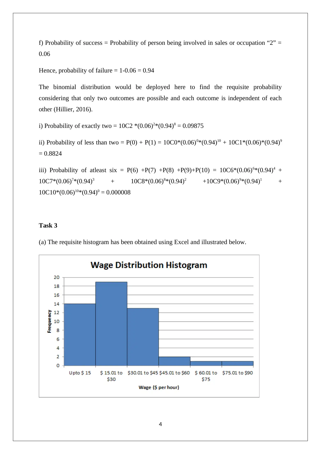
(a) The requisite histogram has been obtained using Excel and illustrated below.
4

From the above histogram, it is apparent that the distribution of wages is non-normal
considering the fact that rightward skew or positive skew is present. This is apparent since the
right tail is significantly longer than the corresponding left tail to the sample mean (Flick,
2015). Further, it also implies that there are certain individuals who are paid a significantly
high wage rate in excess of $ 75 per hour. However, the majority of the individuals are paid
near the lower end as is apparent from the above wage distribution.
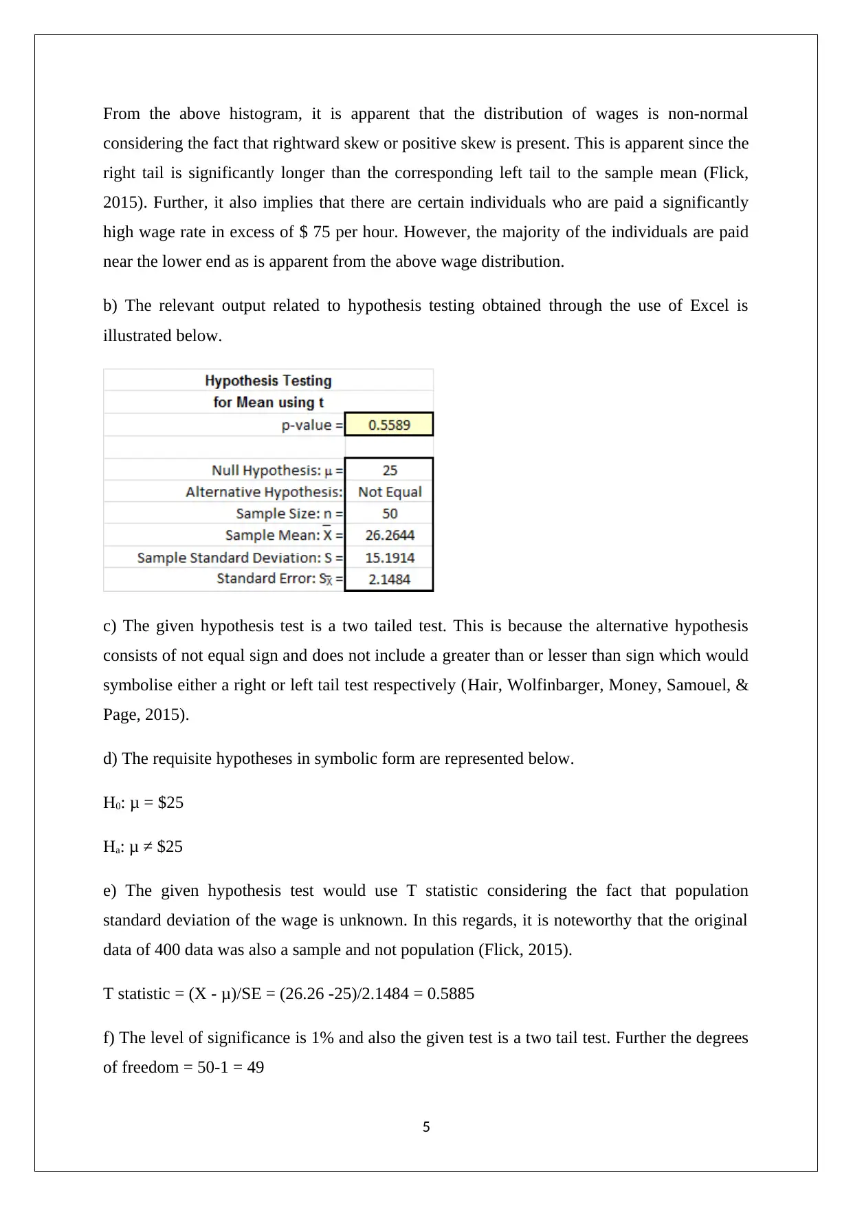
b) The relevant output related to hypothesis testing obtained through the use of Excel is
illustrated below.
c) The given hypothesis test is a two tailed test. This is because the alternative hypothesis
consists of not equal sign and does not include a greater than or lesser than sign which would
symbolise either a right or left tail test respectively (Hair, Wolfinbarger, Money, Samouel, &
Page, 2015).
d) The requisite hypotheses in symbolic form are represented below.
H0: μ = $25
Ha: μ ≠ $25
e) The given hypothesis test would use T statistic considering the fact that population
standard deviation of the wage is unknown. In this regards, it is noteworthy that the original
data of 400 data was also a sample and not population (Flick, 2015).
T statistic = (X - μ)/SE = (26.26 -25)/2.1484 = 0.5885
f) The level of significance is 1% and also the given test is a two tail test. Further the degrees
of freedom = 50-1 = 49
5

The critical values of t statistics based on the above input data amount to -2.68 and 2.68.
g) It is apparent that the calculated t statistic value tends to lie between the critical values i.e.
-2.68 and 2.68. As a result, the null hypothesis would not be rejected. Thus, the alternative
hypothesis cannot be accepted. Hence, it may be concluded that the mean wage is not
different from $ 25 per hour (Hair, Wolfinbarger, Money, Samouel, & Page, 2015).
h) From the above computations, sample mean wage = $ 26.26, Standard error of the sample
mean = $ 2.148
Further, the t statistic would be sued instead of Z since the population standard deviation for
wages is not known. Relevant t value corresponding to 99% confidence level = 2.68
Upper level of 99% confidence interval for mean wage = 26.26 + 2.68*2.148 = $ 32.02
Lower level of 99% confidence interval for mean wage = 26.26 - 2.68*2.148 = $ 20.51
i) Now, since the confidence level has been altered to 95% , hence the critical values would
change. However, there would be no change in the value of T statistic obtained which would
remain the same as earlier. The revised critical values for t are -2.01 and 2.01.
j) It is apparent that the calculated t statistic value tends to lie between the critical values i.e. -
2.01 and 2.01. As a result, the null hypothesis would not be rejected (Eriksson & Kovalainen,
2015). Thus, the alternative hypothesis cannot be accepted. Hence, it may be concluded that
the mean wage is not different from $ 25 per hour.
k) From the above computations, sample mean wage = $ 26.26, Standard error of the sample
mean = $ 2.148
Further, the t statistic would be sued instead of Z since the population standard deviation for
wages is not known. Relevant t value corresponding to 95% confidence level = 2.01
Upper level of 95% confidence interval for mean wage = 26.26 + 2.01*2.148 = $ 30.58
Lower level of 95% confidence interval for mean wage = 26.26 - 2.01*2.148 = $ 21.95
l) The 95% confidence interval computed above implies that there is a 95% likelihood that
the average wage of the population would lie between $ 21.95 per hour and $ 30.58 per hour.
Further, comparing the 95% confidence interval and 99% confidence interval, it is apparent
that higher precision would require a wider confidence interval (Hillier, 2016).
6

Conclusion
The occupation distribution of the selected sample has been obtained and used to compute the
respective probabilities using binomial distribution. Also, in terms of sex, the selected sample
has a majority of females. Further, it has also come to light the wage distribution is non-
normal since there are some individuals who are paid an abnormally high wage. However, the
hypothesis testing suggests that average wage cannot be said to deviate from $ 25 per hour
both at 95% and 99% confidence intervals.
7

References
Eriksson, P. & Kovalainen, A. (2015) Quantitative methods in business research. 3rd ed.
London: Sage Publications.
Flick, U. (2015) Introducing research methodology: A beginner's guide to doing a research
project. 4th ed. New York: Sage Publications
Hair, J. F., Wolfinbarger, M., Money, A. H., Samouel, P., & Page, M. J. (2015) Essentials of
business research methods. 2nd ed. New York: Routledge.
Hillier, F. (2016) Introduction to Operations Research. 6th ed. New York: McGraw Hill
Publications.
8