STAT603: Forecasting - Desklib

This article discusses the quarterly sales of beer in New Zealand over an 8-year period and the forecasting of the next two years using exponential smoothing, Holt’s Linear Trend, and Damped Trend. It also covers ACF and PACF plots, ARIMA models, and ETS methods for forecasting. The article provides R-codes and plots for each method and model. The appropriate ARIMA model for the series is given as (1,1,4).

Running Head: STAT603: FORECASTING
STAT603
Forecasting
Name of the Student
Name of the University
Author Note

1STAT603: FORECASTING
Table of Contents
Task 1...............................................................................................................................................2
Part A...........................................................................................................................................2
Part B...........................................................................................................................................2
Part C...........................................................................................................................................5
Task 2...............................................................................................................................................6
Part A...........................................................................................................................................6
Part B...........................................................................................................................................8
Task 3...............................................................................................................................................9
Part A...........................................................................................................................................9
Part B.........................................................................................................................................10
Part C.........................................................................................................................................10
Part D.............................................................................................................................................10
Part E.........................................................................................................................................11
Part F..........................................................................................................................................12
Part G.........................................................................................................................................13
Part H.........................................................................................................................................13

2STAT603: FORECASTING
Task 1
Part A
The quarterly sales of beer (in million litres) in New Zealand over the 8-year period from
2010 to 2017 is given in the following figure 1.1. It can be seen clearly from the figure that the
sale of beer is highest in the first and the fourth quarter every year and decreases in the second
and the third quarters. Thus, it can be said that the data is seasonal. The R-Code for the plot is
given in the following table 1.1.
Table 1.1: R code for plotting the sales of beer over time
timeseries<-ts(data, frequency = 4, start = c(2010,1))
timeseries
plot.ts(timeseries)
Figure 1.1: Time series plot of total beer sales over time
Part B
The forecast of the next two years of 2018 and 2019 with the help of exponential
smoothing method, Holt’s Linear Trend and Damped Trend are given in figures 1.2, 1.3 and 1.4

3STAT603: FORECASTING
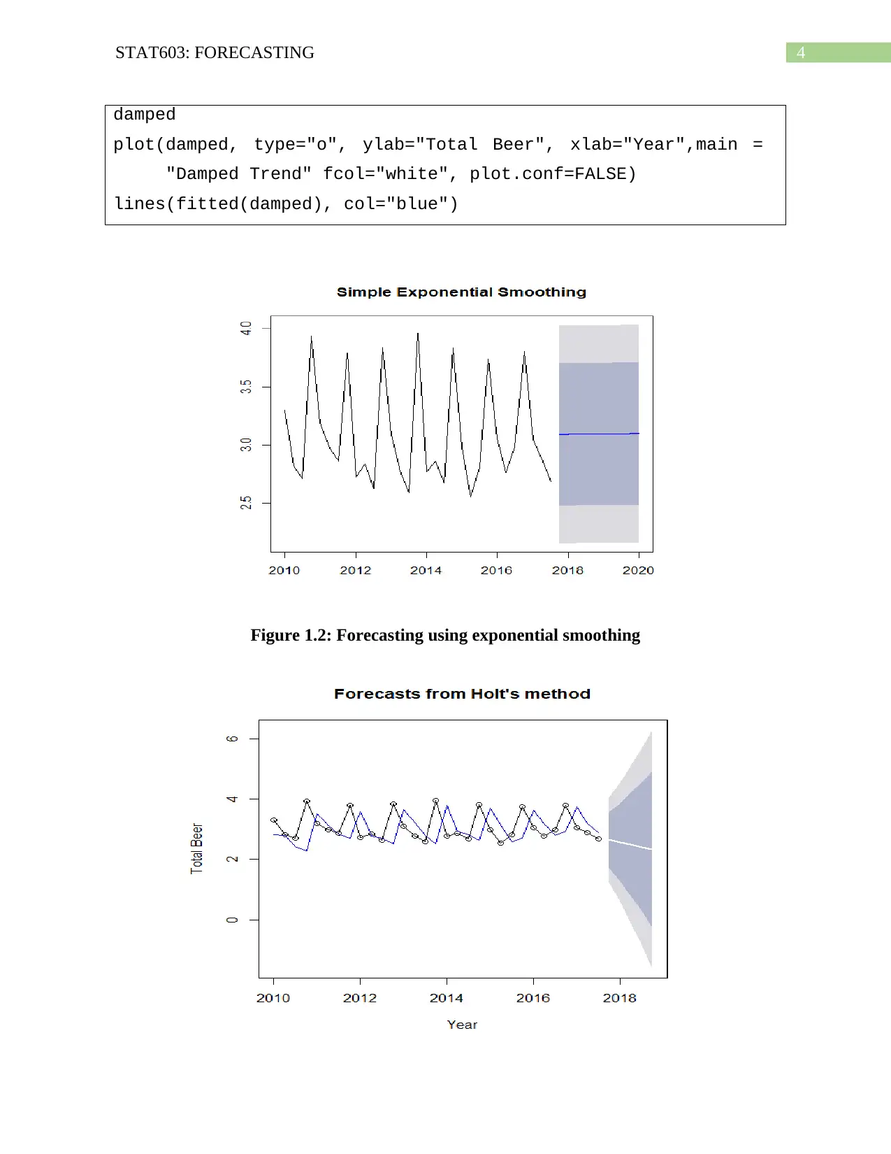
respectively. It can be observed from the figures that the simple exponential smoothing
eliminates the effects of seasonality from the data and gives the results which might not be an
accurate forecasting model.
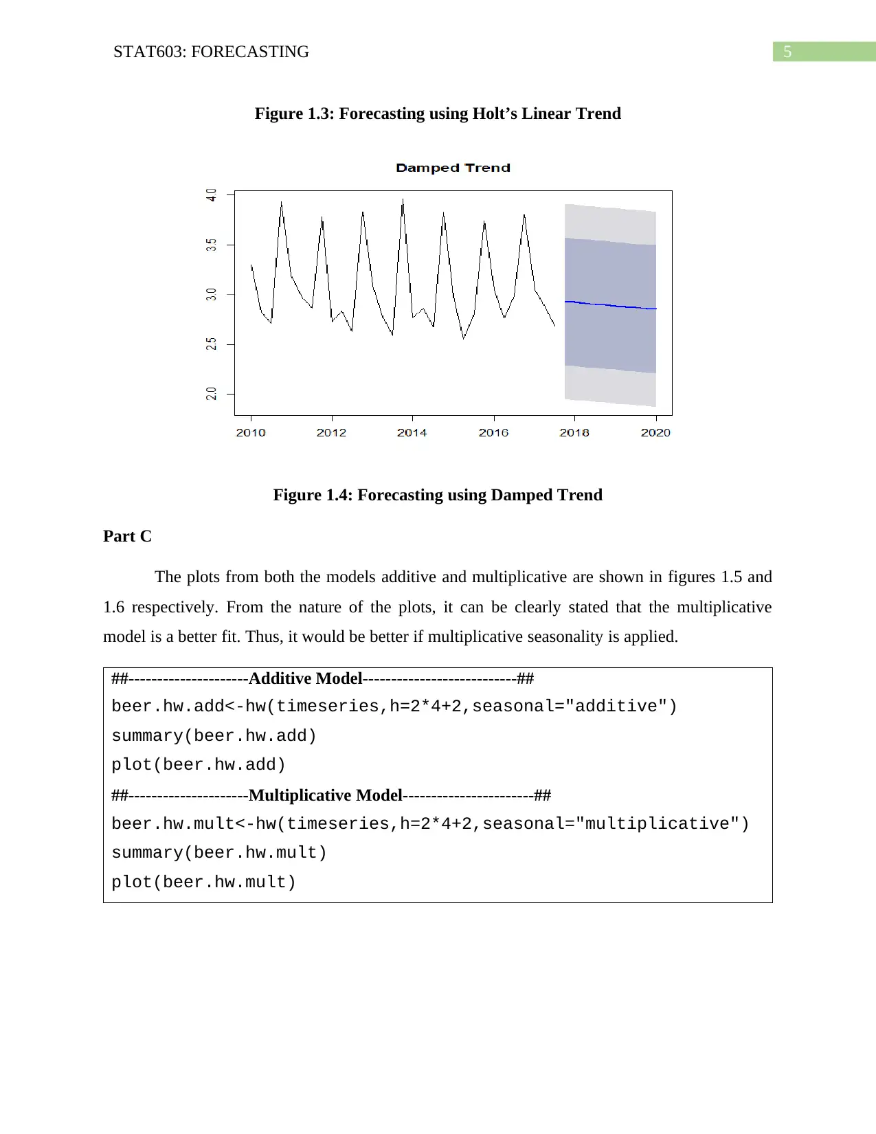
The holts linear trend method can explain the effects of seasonality in the data and create
the forecasting model accordingly. On the other hand, the damped trend method shows that the
trend is gradually decomposing, which might also not be a proper explanation of the data as not
always the data will be decomposing gradually.
Thus, it can be said that the Holt’s linear trend method is a better prediction and
forecasting model than the other three developed models. The R-Codes for the three models are
provided in table 1.2.
Table 1.2: R-Codes for Exponential Smoothing, Holt’s Linear Trend and Damped Trend
Model
##--------------Simple Exponential Smoothing----------------------##
simpleexp<-holt(timeseries, h=2*4+2)
simpleexp
plot(simpleexp,main="Simple Exponential Smoothing")
accuracy(simpleexp)
##--------------Holt Linear Trend----------------------##
holt <- holt(timeseries, alpha=0.8, beta=0.2,lead = 2, damped =
FALSE,
initial="simple", h=2*4+2,plot=TRUE)
holt
plot(holt, type="o", ylab="Total Beer", xlab="Year",
fcol="white", plot.conf=FALSE)
lines(fitted(holt), col="blue")
##--------------Damped Trend----------------------##
damped <- holt(timeseries, alpha=0.8, beta=0.2,lead = 2, damped
= FALSE, initial="simple", h=5,plot=TRUE)

4STAT603: FORECASTING
damped
plot(damped, type="o", ylab="Total Beer", xlab="Year",main =
"Damped Trend" fcol="white", plot.conf=FALSE)
lines(fitted(damped), col="blue")
Figure 1.2: Forecasting using exponential smoothing

5STAT603: FORECASTING
Figure 1.3: Forecasting using Holt’s Linear Trend
Figure 1.4: Forecasting using Damped Trend
Part C
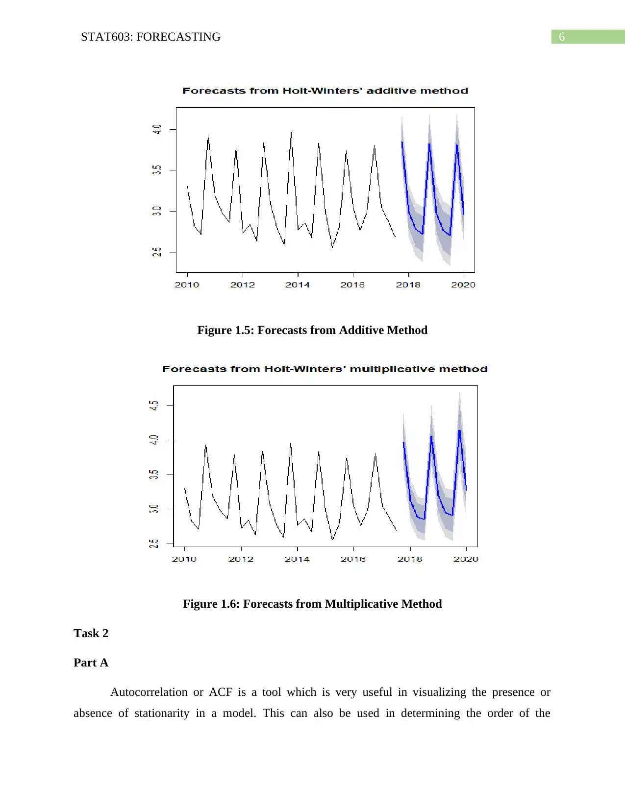
The plots from both the models additive and multiplicative are shown in figures 1.5 and
1.6 respectively. From the nature of the plots, it can be clearly stated that the multiplicative
model is a better fit. Thus, it would be better if multiplicative seasonality is applied.
##---------------------Additive Model---------------------------##
beer.hw.add<-hw(timeseries,h=2*4+2,seasonal="additive")
summary(beer.hw.add)
plot(beer.hw.add)
##---------------------Multiplicative Model-----------------------##
beer.hw.mult<-hw(timeseries,h=2*4+2,seasonal="multiplicative")
summary(beer.hw.mult)
plot(beer.hw.mult)

6STAT603: FORECASTING
Figure 1.5: Forecasts from Additive Method
Figure 1.6: Forecasts from Multiplicative Method
Task 2
Part A
Autocorrelation or ACF is a tool which is very useful in visualizing the presence or
absence of stationarity in a model. This can also be used in determining the order of the

7STAT603: FORECASTING
parameters of the ARIMA model. The correlation between the series and its lags are visualized
with the help of the ACF plot. A correlation between the series and its lags indicates that the
series is not stationary and trend or seasonality exists over time.
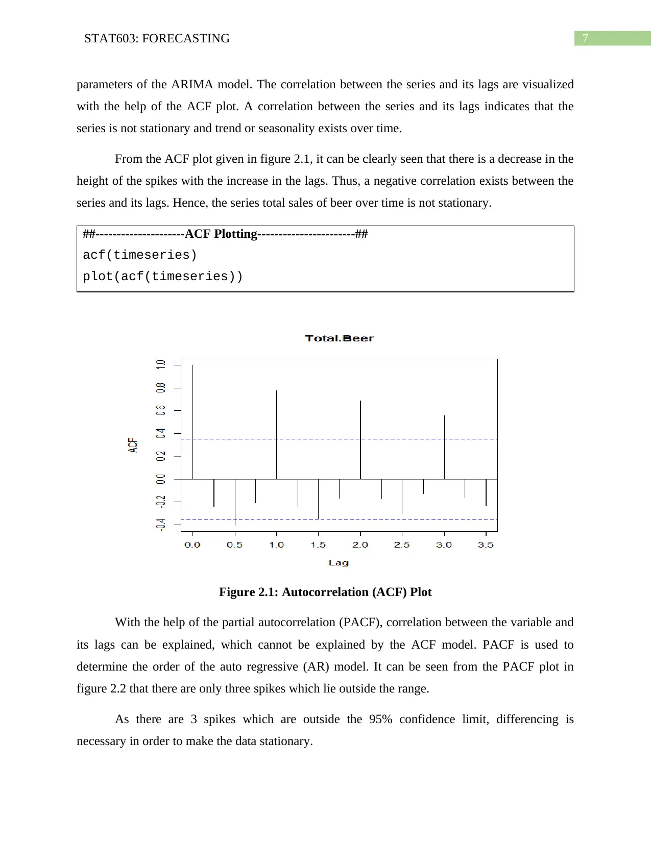
From the ACF plot given in figure 2.1, it can be clearly seen that there is a decrease in the
height of the spikes with the increase in the lags. Thus, a negative correlation exists between the
series and its lags. Hence, the series total sales of beer over time is not stationary.
##---------------------ACF Plotting-----------------------##
acf(timeseries)
plot(acf(timeseries))
Figure 2.1: Autocorrelation (ACF) Plot
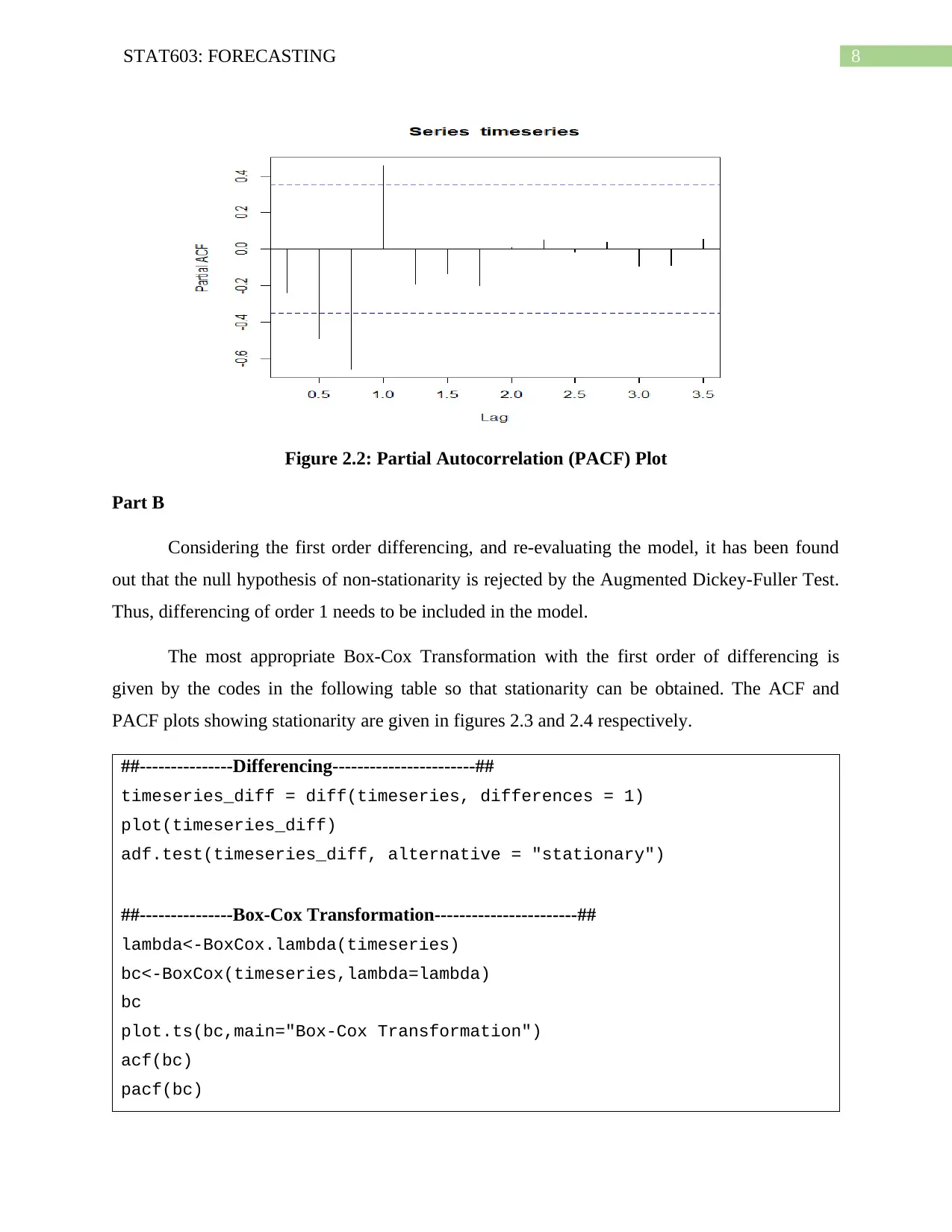
With the help of the partial autocorrelation (PACF), correlation between the variable and
its lags can be explained, which cannot be explained by the ACF model. PACF is used to
determine the order of the auto regressive (AR) model. It can be seen from the PACF plot in
figure 2.2 that there are only three spikes which lie outside the range.
As there are 3 spikes which are outside the 95% confidence limit, differencing is
necessary in order to make the data stationary.

8STAT603: FORECASTING
Figure 2.2: Partial Autocorrelation (PACF) Plot
Part B
Considering the first order differencing, and re-evaluating the model, it has been found
out that the null hypothesis of non-stationarity is rejected by the Augmented Dickey-Fuller Test.
Thus, differencing of order 1 needs to be included in the model.
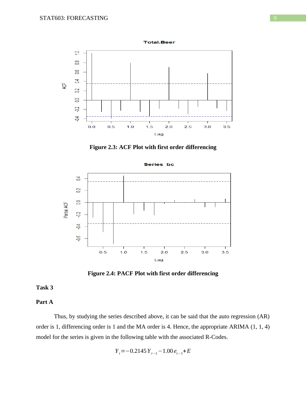
The most appropriate Box-Cox Transformation with the first order of differencing is
given by the codes in the following table so that stationarity can be obtained. The ACF and
PACF plots showing stationarity are given in figures 2.3 and 2.4 respectively.
##---------------Differencing-----------------------##
timeseries_diff = diff(timeseries, differences = 1)
plot(timeseries_diff)
adf.test(timeseries_diff, alternative = "stationary")
##---------------Box-Cox Transformation-----------------------##
lambda<-BoxCox.lambda(timeseries)
bc<-BoxCox(timeseries,lambda=lambda)
bc
plot.ts(bc,main="Box-Cox Transformation")
acf(bc)
pacf(bc)

9STAT603: FORECASTING
Figure 2.3: ACF Plot with first order differencing
Figure 2.4: PACF Plot with first order differencing
Task 3
Part A
Thus, by studying the series described above, it can be said that the auto regression (AR)
order is 1, differencing order is 1 and the MA order is 4. Hence, the appropriate ARIMA (1, 1, 4)
model for the series is given in the following table with the associated R-Codes.
Y t =−0.2145 Y t −1 −1.00 et −1+E

10STAT603: FORECASTING
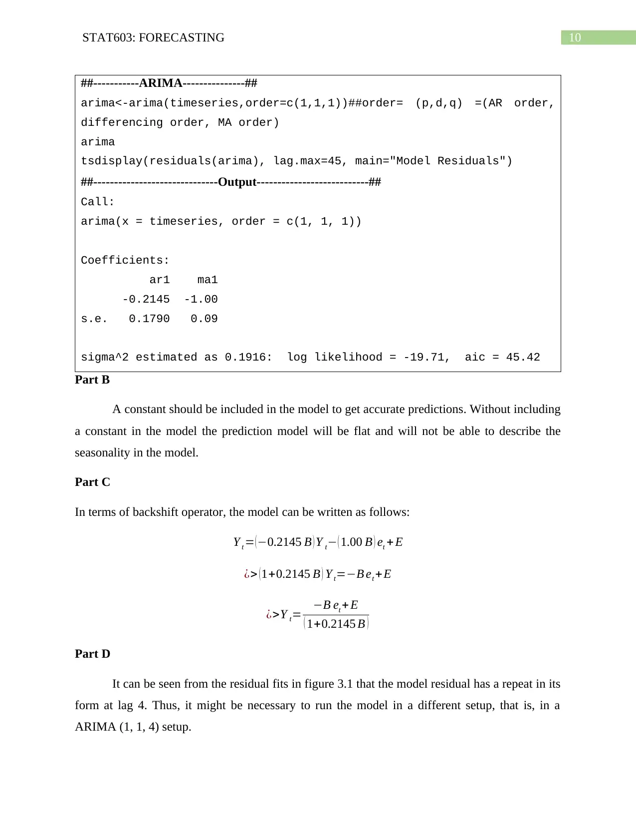
##-----------ARIMA---------------##
arima<-arima(timeseries,order=c(1,1,1))##order= (p,d,q) =(AR order,
differencing order, MA order)
arima
tsdisplay(residuals(arima), lag.max=45, main="Model Residuals")
##------------------------------Output---------------------------##
Call:
arima(x = timeseries, order = c(1, 1, 1))
Coefficients:
ar1 ma1
-0.2145 -1.00
s.e. 0.1790 0.09
sigma^2 estimated as 0.1916: log likelihood = -19.71, aic = 45.42
Part B
A constant should be included in the model to get accurate predictions. Without including
a constant in the model the prediction model will be flat and will not be able to describe the
seasonality in the model.
Part C
In terms of backshift operator, the model can be written as follows:
Y t = (−0.2145 B ) Y t− ( 1.00 B ) et + E
¿> ( 1+0.2145 B ) Y t=−B et +E
¿>Y t= −B et + E
( 1+0.2145 B )
Part D
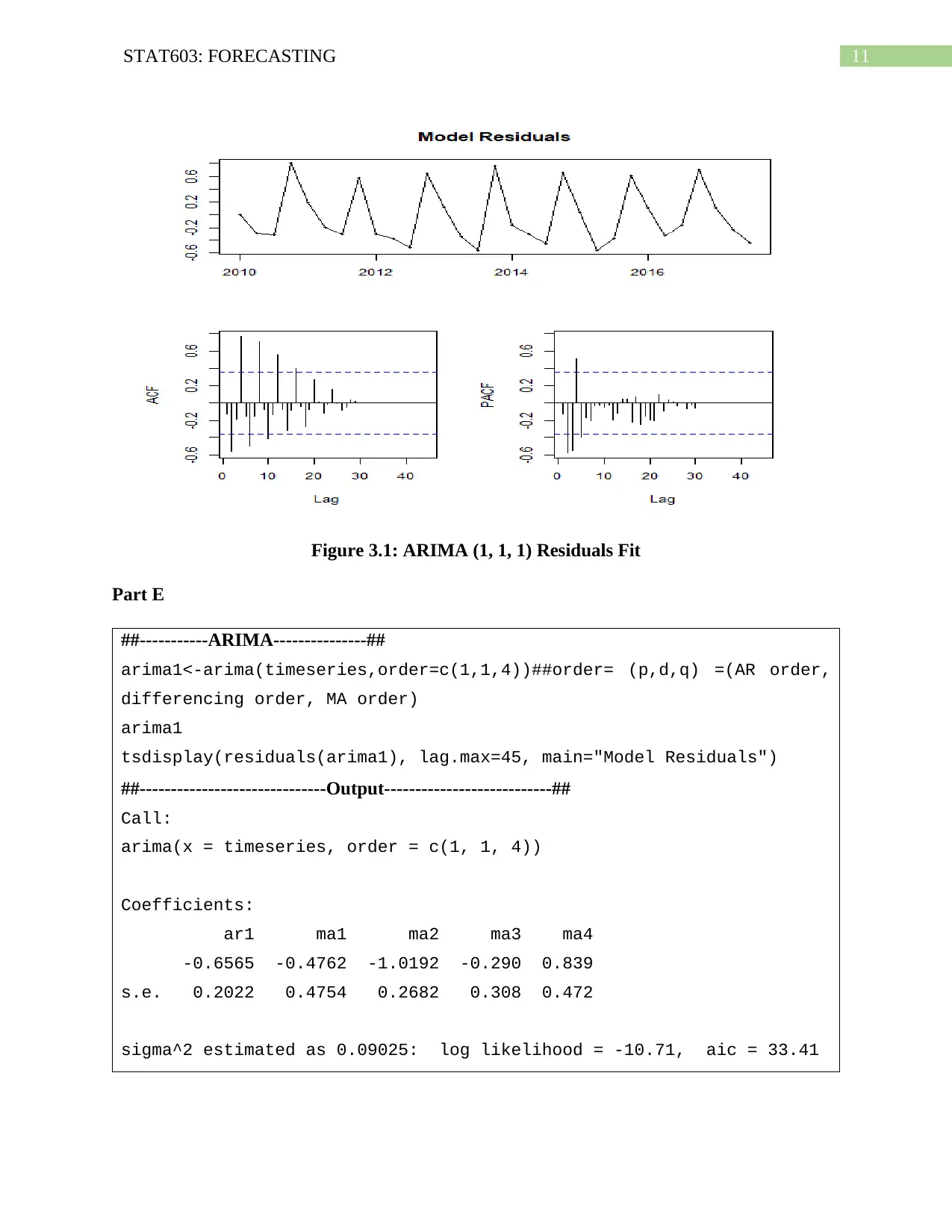
It can be seen from the residual fits in figure 3.1 that the model residual has a repeat in its
form at lag 4. Thus, it might be necessary to run the model in a different setup, that is, in a
ARIMA (1, 1, 4) setup.

11STAT603: FORECASTING
Figure 3.1: ARIMA (1, 1, 1) Residuals Fit
Part E
##-----------ARIMA---------------##
arima1<-arima(timeseries,order=c(1,1,4))##order= (p,d,q) =(AR order,
differencing order, MA order)
arima1
tsdisplay(residuals(arima1), lag.max=45, main="Model Residuals")
##------------------------------Output---------------------------##
Call:
arima(x = timeseries, order = c(1, 1, 4))
Coefficients:
ar1 ma1 ma2 ma3 ma4
-0.6565 -0.4762 -1.0192 -0.290 0.839
s.e. 0.2022 0.4754 0.2682 0.308 0.472
sigma^2 estimated as 0.09025: log likelihood = -10.71, aic = 33.41

12STAT603: FORECASTING
Figure 3.1: ARIMA (1, 1, 4) Residuals Fit
Part F
fcast <- forecast(arima1, h=30)
plot(fcast)
Figure 3.3: Forecast from ARIMA (1, 1, 4) Model

13STAT603: FORECASTING
Part G
There are some differences in the results of ARIMA ( ) and AUTO.ARIMA ( ) models.
The auto.arima ( ) model selects the parameters that is best for the model on its own. Thus, the
auto.arima ( ) model is said to be a better model that arima ( ).
arima2<-auto.arima(timeseries,seasonal=FALSE)
arima2
tsdisplay(residuals(arima2), lag.max=45, main="Model Residuals")
##---------------Output------------------##
Series: timeseries
ARIMA(0,0,0) with non-zero mean
Coefficients:
mean
3.0811
s.e. 0.0797
sigma^2 estimated as 0.2034: log likelihood=-18.8
AIC=41.59 AICc=42.02 BIC=44.46
Part H
By comparing the ETS method with the ARIMA method, it can be clearly seen that
ARIMA is a much better prediction model than the ETS model.