Travel Company Forecasting

This assignment involves applying the additive method of forecasting to predict the number of excursions sold by a travel company in 2018. The company has four quarters (Q1, Q2, Q3, Q4) with different sales patterns. Historical data is provided for each quarter, and the task is to use this information to forecast future trends using time series analysis. The assignment also includes references to relevant studies on forecasting and time series analysis.

STATICS PROJECT

Table of Contents
QUESTION 1...................................................................................................................................1
(A)....................................................................................................................................................1
1..............................................................................................................................................1
2..............................................................................................................................................1
3..............................................................................................................................................1
(B) ...................................................................................................................................................2
1..............................................................................................................................................2
2..............................................................................................................................................3
3..............................................................................................................................................3
4..............................................................................................................................................4
QUESTION 2...................................................................................................................................4
(A)...........................................................................................................................................4
(B)...........................................................................................................................................6
REFERENCES................................................................................................................................8

QUESTION 1
(A)
1
Chart first that reflects lost luggage in first 6 months in the year 2015 show that number of pieces
of luggage from Jan to Feb has increased whereas in the March month it has decreased. After
that in the month April it has been increased but in May month it again number of pieces has
been decreased that enhanced again in June (Harvey, Chastin and Skelton, 2015). That reflects
its fluctuation is too high. On other hand in the year 2016 number of pieces of luggage have
decreased continuously in every month as compare to year 2015.
2
Both two graphs are unable to show true reflection about what happened because both these
graphs show their own performance in particular year, there is no comparison between two years
data.
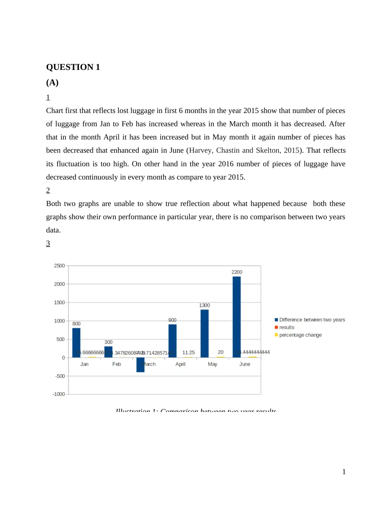
3
Illustration 1: Comparison between two year results
1

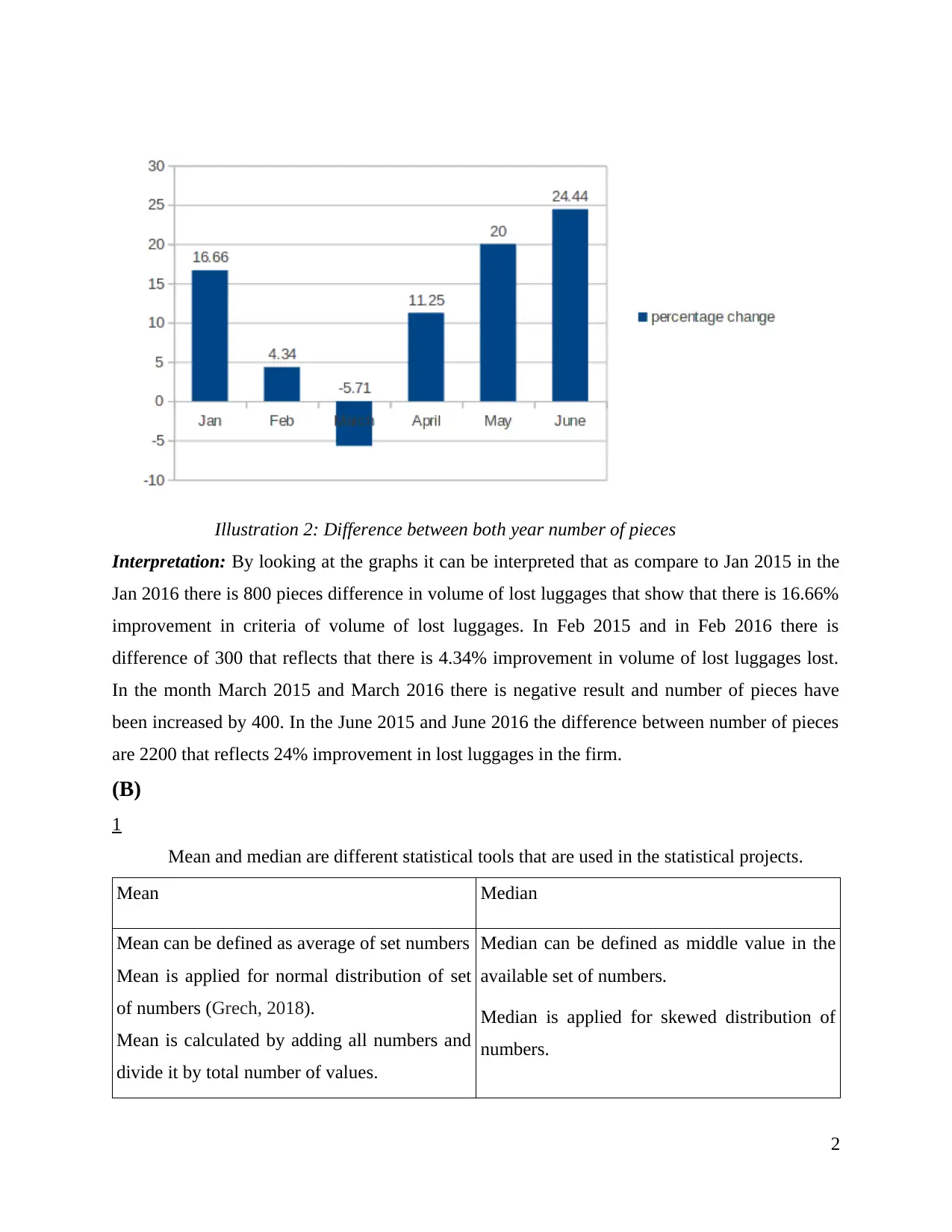
Illustration 2: Difference between both year number of pieces
Interpretation: By looking at the graphs it can be interpreted that as compare to Jan 2015 in the
Jan 2016 there is 800 pieces difference in volume of lost luggages that show that there is 16.66%
improvement in criteria of volume of lost luggages. In Feb 2015 and in Feb 2016 there is
difference of 300 that reflects that there is 4.34% improvement in volume of lost luggages lost.
In the month March 2015 and March 2016 there is negative result and number of pieces have
been increased by 400. In the June 2015 and June 2016 the difference between number of pieces
are 2200 that reflects 24% improvement in lost luggages in the firm.
(B)
1
Mean and median are different statistical tools that are used in the statistical projects.
Mean Median
Mean can be defined as average of set numbers
Mean is applied for normal distribution of set
of numbers (Grech, 2018).
Mean is calculated by adding all numbers and
divide it by total number of values.
Median can be defined as middle value in the
available set of numbers.
Median is applied for skewed distribution of
numbers.
2

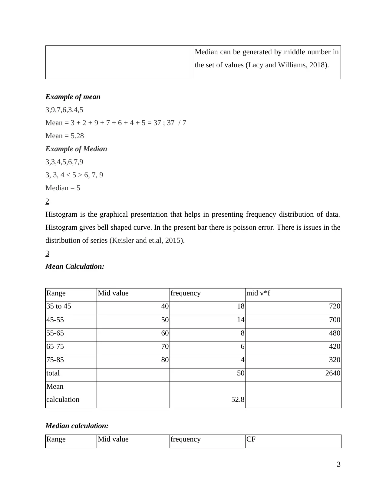
Median can be generated by middle number in
the set of values (Lacy and Williams, 2018).
Example of mean
3,9,7,6,3,4,5
Mean = 3 + 2 + 9 + 7 + 6 + 4 + 5 = 37 ; 37 / 7
Mean = 5.28
Example of Median
3,3,4,5,6,7,9
3, 3, 4 < 5 > 6, 7, 9
Median = 5
2
Histogram is the graphical presentation that helps in presenting frequency distribution of data.
Histogram gives bell shaped curve. In the present bar there is poisson error. There is issues in the
distribution of series (Keisler and et.al, 2015).
3
Mean Calculation:
Range Mid value frequency mid v*f
35 to 45 40 18 720
45-55 50 14 700
55-65 60 8 480
65-75 70 6 420
75-85 80 4 320
total 50 2640
Mean
calculation 52.8
Median calculation:
Range Mid value frequency CF
3

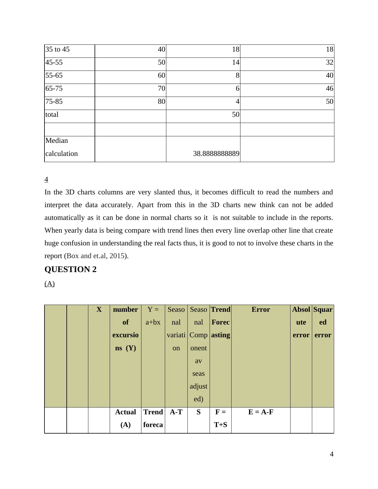
35 to 45 40 18 18
45-55 50 14 32
55-65 60 8 40
65-75 70 6 46
75-85 80 4 50
total 50
Median
calculation 38.8888888889
4
In the 3D charts columns are very slanted thus, it becomes difficult to read the numbers and
interpret the data accurately. Apart from this in the 3D charts new think can not be added
automatically as it can be done in normal charts so it is not suitable to include in the reports.
When yearly data is being compare with trend lines then every line overlap other line that create
huge confusion in understanding the real facts thus, it is good to not to involve these charts in the
report (Box and et.al, 2015).
QUESTION 2
(A)
X number
of
excursio
ns (Y)
Y =
a+bx
Seaso
nal
variati
on
Seaso
nal
Comp
onent
av
seas
adjust
ed)
Trend
Forec
asting
Error Absol
ute
error
Squar
ed
error
Actual
(A)
Trend
foreca
A-T S F =
T+S
E = A-F
4

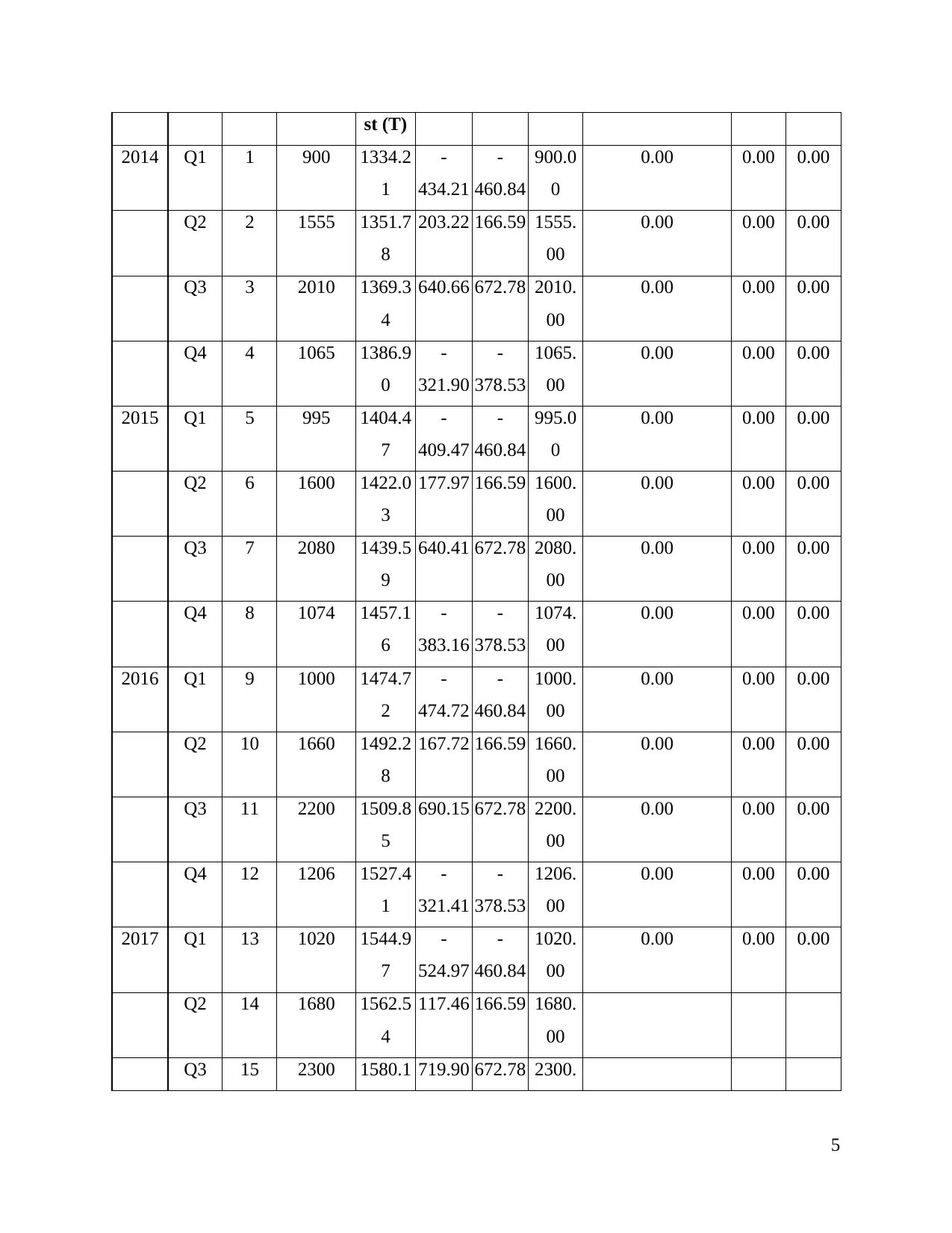
st (T)
2014 Q1 1 900 1334.2
1
-
434.21
-
460.84
900.0
0
0.00 0.00 0.00
Q2 2 1555 1351.7
8
203.22 166.59 1555.
00
0.00 0.00 0.00
Q3 3 2010 1369.3
4
640.66 672.78 2010.
00
0.00 0.00 0.00
Q4 4 1065 1386.9
0
-
321.90
-
378.53
1065.
00
0.00 0.00 0.00
2015 Q1 5 995 1404.4
7
-
409.47
-
460.84
995.0
0
0.00 0.00 0.00
Q2 6 1600 1422.0
3
177.97 166.59 1600.
00
0.00 0.00 0.00
Q3 7 2080 1439.5
9
640.41 672.78 2080.
00
0.00 0.00 0.00
Q4 8 1074 1457.1
6
-
383.16
-
378.53
1074.
00
0.00 0.00 0.00
2016 Q1 9 1000 1474.7
2
-
474.72
-
460.84
1000.
00
0.00 0.00 0.00
Q2 10 1660 1492.2
8
167.72 166.59 1660.
00
0.00 0.00 0.00
Q3 11 2200 1509.8
5
690.15 672.78 2200.
00
0.00 0.00 0.00
Q4 12 1206 1527.4
1
-
321.41
-
378.53
1206.
00
0.00 0.00 0.00
2017 Q1 13 1020 1544.9
7
-
524.97
-
460.84
1020.
00
0.00 0.00 0.00
Q2 14 1680 1562.5
4
117.46 166.59 1680.
00
Q3 15 2300 1580.1 719.90 672.78 2300.
5

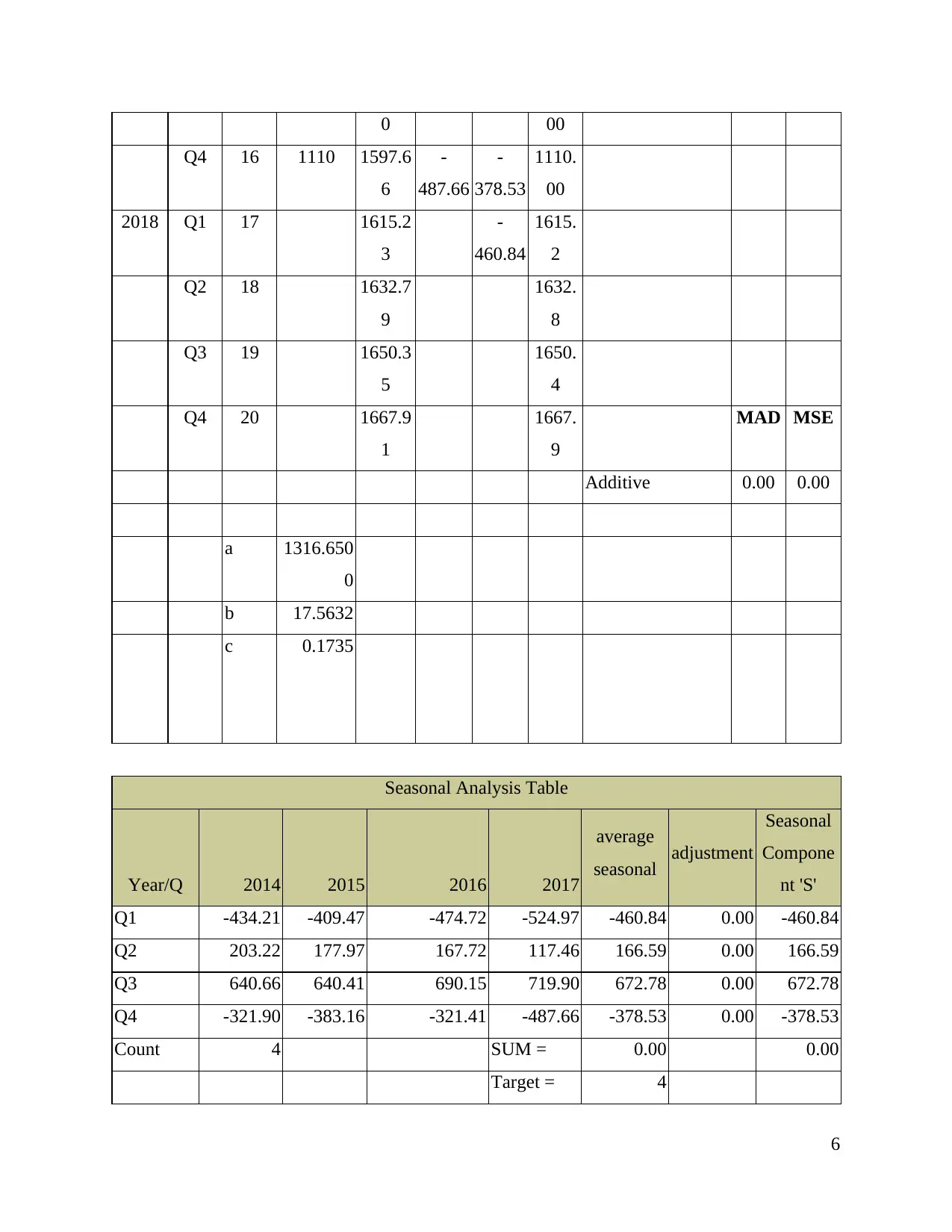
0 00
Q4 16 1110 1597.6
6
-
487.66
-
378.53
1110.
00
2018 Q1 17 1615.2
3
-
460.84
1615.
2
Q2 18 1632.7
9
1632.
8
Q3 19 1650.3
5
1650.
4
Q4 20 1667.9
1
1667.
9
MAD MSE
Additive 0.00 0.00
a 1316.650
0
b 17.5632
c 0.1735
Seasonal Analysis Table
Year/Q 2014 2015 2016 2017
average
seasonal adjustment
Seasonal
Compone
nt 'S'
Q1 -434.21 -409.47 -474.72 -524.97 -460.84 0.00 -460.84
Q2 203.22 177.97 167.72 117.46 166.59 0.00 166.59
Q3 640.66 640.41 690.15 719.90 672.78 0.00 672.78
Q4 -321.90 -383.16 -321.41 -487.66 -378.53 0.00 -378.53
Count 4 SUM = 0.00 0.00
Target = 4
6

Adjustment
s =
0.00
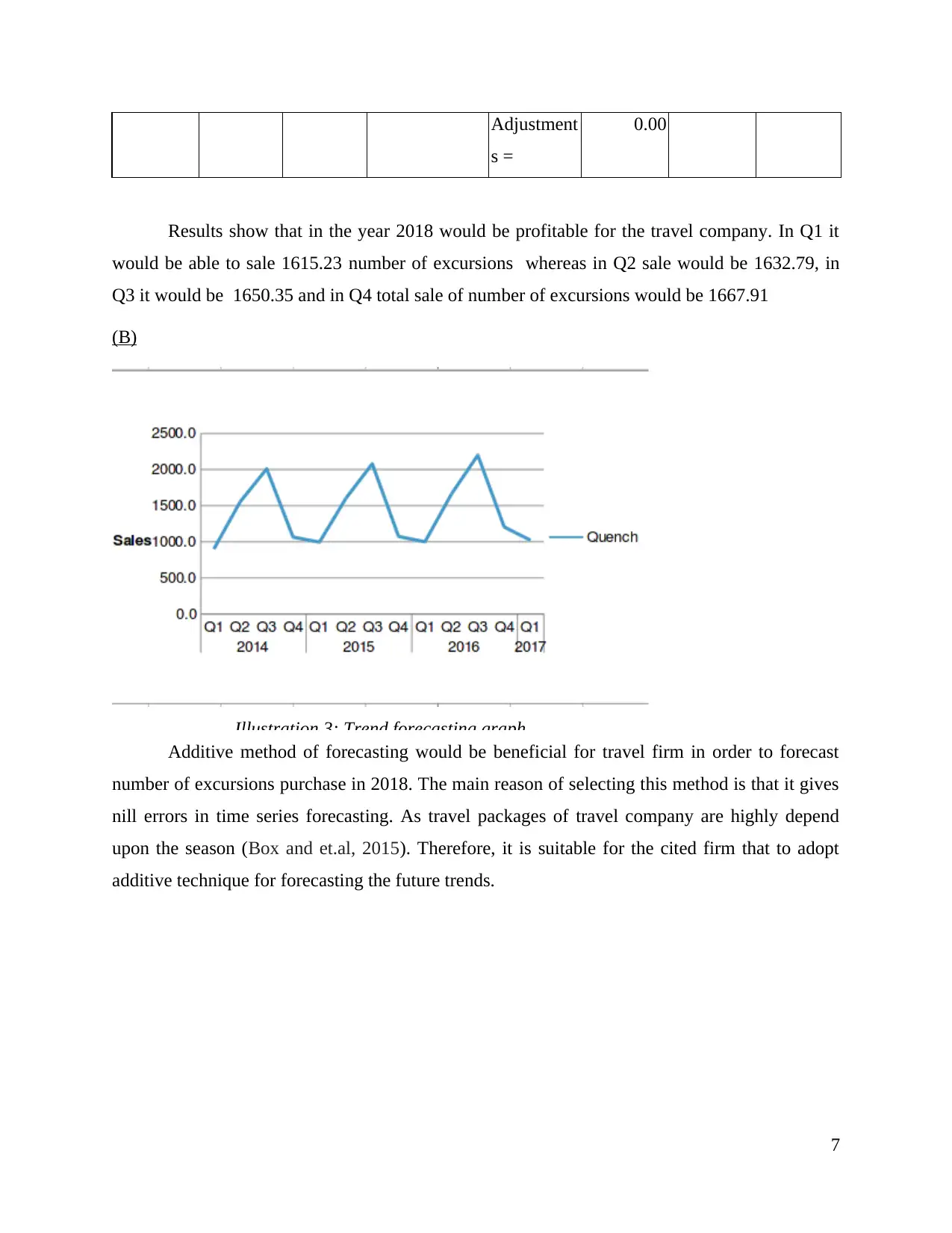
Results show that in the year 2018 would be profitable for the travel company. In Q1 it
would be able to sale 1615.23 number of excursions whereas in Q2 sale would be 1632.79, in
Q3 it would be 1650.35 and in Q4 total sale of number of excursions would be 1667.91
(B)
Illustration 3: Trend forecasting graph
Additive method of forecasting would be beneficial for travel firm in order to forecast
number of excursions purchase in 2018. The main reason of selecting this method is that it gives
nill errors in time series forecasting. As travel packages of travel company are highly depend
upon the season (Box and et.al, 2015). Therefore, it is suitable for the cited firm that to adopt
additive technique for forecasting the future trends.
7

REFERENCES
Box, G. E. and et.al., 2015. Time series analysis: forecasting and control. John Wiley & Sons.
Chatfield, C., 2016. The analysis of time series: an introduction. CRC press.
Grech, V., 2018. WASP (Write a Scientific Paper) using Excel–5: Quartiles and standard
deviation. Early human development.
Harvey, J. A., Chastin, S. F. and Skelton, D. A., 2015. How sedentary are older people? A
systematic review of the amount of sedentary behavior. Journal of aging and physical
activity. 23(3). pp.471-487.
Keisler, R. and et.al., 2015. Measurements of sub-degree B-mode polarization in the cosmic
microwave background from 100 square degrees of SPTpol data. The Astrophysical
Journal. 807(2). pp.151.
Lacy, A. C. and Williams, S. M., 2018. Measurement and evaluation in physical education and
exercise science. Routledge.
8