Statistical Analysis and Interpretation of Data

This report delves into the fundamental concepts of statistical analysis, exploring various techniques and their applications in data interpretation. It covers frequency distributions, regression analysis, ANOVA, and correlation, providing a comprehensive understanding of these statistical tools. The report utilizes real-world examples to illustrate the practical implications of these methods, enabling readers to grasp the significance of statistical analysis in decision-making processes.

Statistics Assignment
1

Table of Contents
Introduction....................................................................................................................................2
Task 1..............................................................................................................................................3
Task 2..............................................................................................................................................5
Task 3..............................................................................................................................................6
Task 4..............................................................................................................................................7
Conclusion......................................................................................................................................9
References.....................................................................................................................................10
2

Introduction
The given report covers the various aspects relating to statistical accounting as well as some
branch of studies relating to research methodology. Since it is a broader concept, only major
aspects and concepts relating to these branches of studies have been covered. An attempt has
been made to understand the practical scenario and situation of the given circumstances so that
reasonable assumptions can be drawn. This will help to draw a better conclusion. It depends on
the user or reader of the report how he interprets the conclusion of the report. As it requires
calculation, it is a study of collecting, analyzing, interpreting and accordingly summarizing data.
In this manner, by applying statistical tools and techniques of statistics, the strategic or top-level
managers or executives can take crucial decisions. In this manner, any business enterprise can
achieve strategic competitive advantage and can acquire the market share.
3

Task 1
(a)
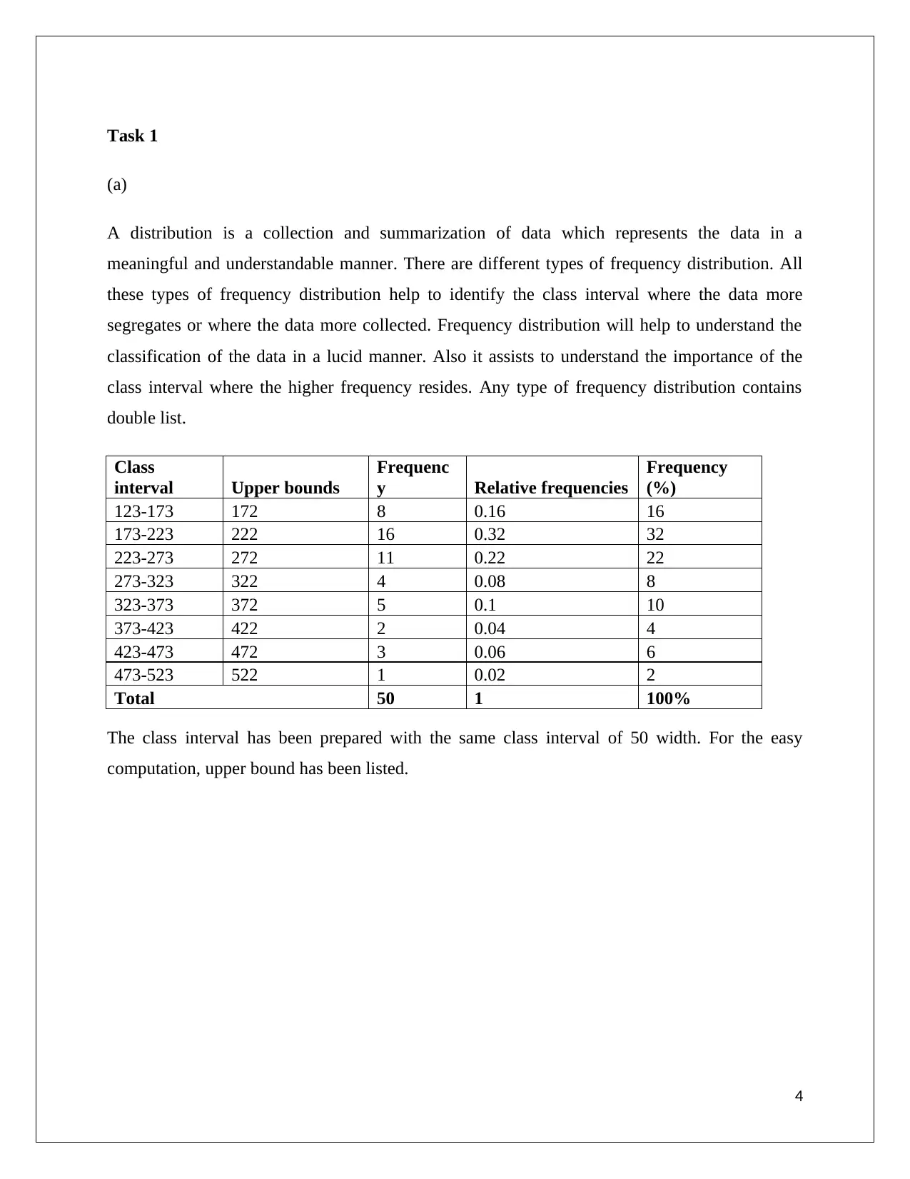
A distribution is a collection and summarization of data which represents the data in a
meaningful and understandable manner. There are different types of frequency distribution. All
these types of frequency distribution help to identify the class interval where the data more
segregates or where the data more collected. Frequency distribution will help to understand the
classification of the data in a lucid manner. Also it assists to understand the importance of the
class interval where the higher frequency resides. Any type of frequency distribution contains
double list.
Class
interval Upper bounds
Frequenc
y Relative frequencies
Frequency
(%)
123-173 172 8 0.16 16
173-223 222 16 0.32 32
223-273 272 11 0.22 22
273-323 322 4 0.08 8
323-373 372 5 0.1 10
373-423 422 2 0.04 4
423-473 472 3 0.06 6
473-523 522 1 0.02 2
Total 50 1 100%
The class interval has been prepared with the same class interval of 50 width. For the easy
computation, upper bound has been listed.
4

(b)
1 2 3 4 5 6 7 8
0
5
10
15
20
25
30
35
Class intervals
Furniture order value
Histogram showing relative
frequency of furniture order
value
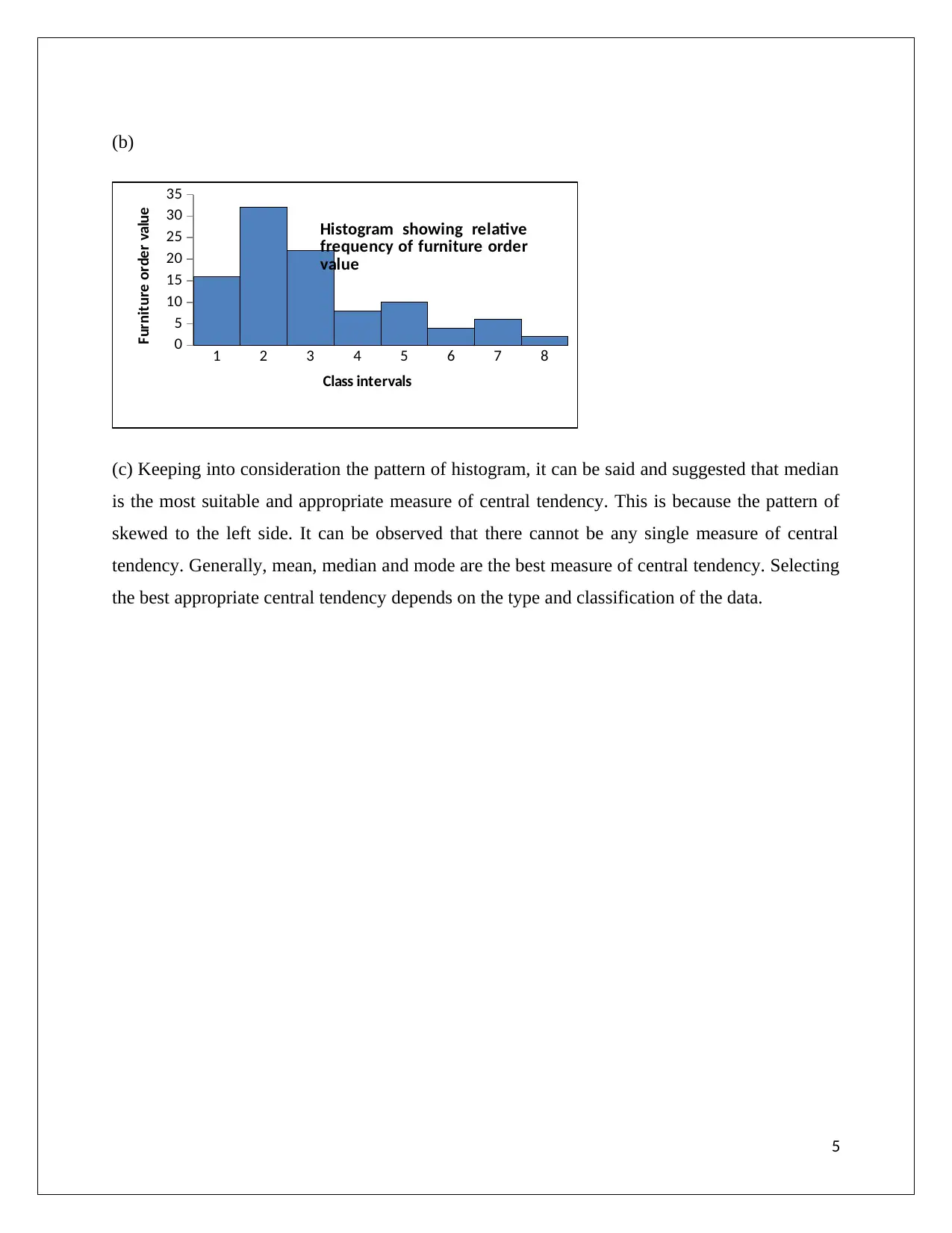
(c) Keeping into consideration the pattern of histogram, it can be said and suggested that median
is the most suitable and appropriate measure of central tendency. This is because the pattern of
skewed to the left side. It can be observed that there cannot be any single measure of central
tendency. Generally, mean, median and mode are the best measure of central tendency. Selecting
the best appropriate central tendency depends on the type and classification of the data.
5

Task 2
ANOVA Table
Sources of Variation Degree of
freedom Sum of Square Mean Square F
Regression 1 5,048.82 5,048.82 74.14
Error 46 3,132.66 68.10
Total 47 8,181.48
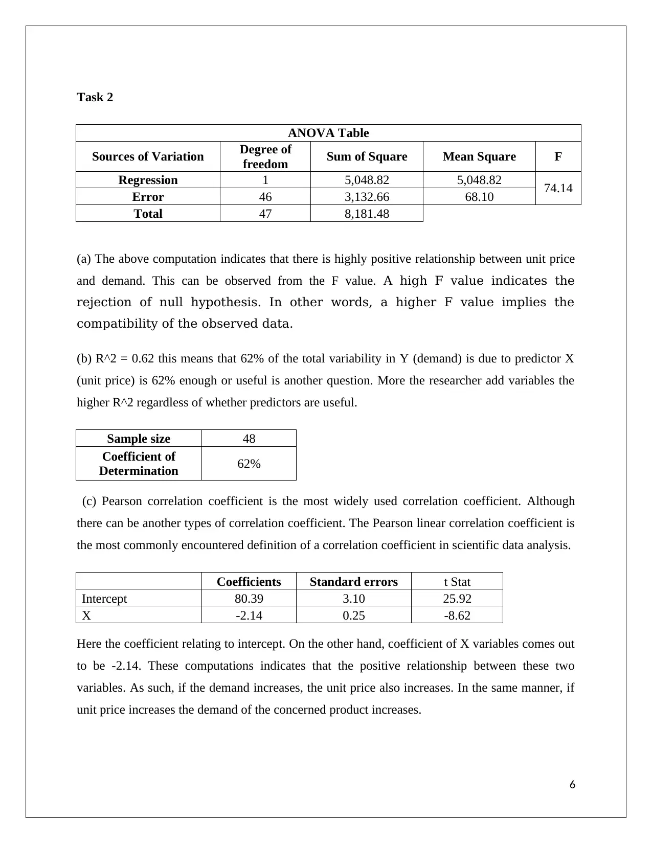
(a) The above computation indicates that there is highly positive relationship between unit price
and demand. This can be observed from the F value. A high F value indicates the
rejection of null hypothesis. In other words, a higher F value implies the
compatibility of the observed data.
(b) R^2 = 0.62 this means that 62% of the total variability in Y (demand) is due to predictor X
(unit price) is 62% enough or useful is another question. More the researcher add variables the
higher R^2 regardless of whether predictors are useful.
Sample size 48
Coefficient of
Determination 62%
(c) Pearson correlation coefficient is the most widely used correlation coefficient. Although
there can be another types of correlation coefficient. The Pearson linear correlation coefficient is
the most commonly encountered definition of a correlation coefficient in scientific data analysis.
Coefficients Standard errors t Stat
Intercept 80.39 3.10 25.92
X -2.14 0.25 -8.62
Here the coefficient relating to intercept. On the other hand, coefficient of X variables comes out
to be -2.14. These computations indicates that the positive relationship between these two
variables. As such, if the demand increases, the unit price also increases. In the same manner, if
unit price increases the demand of the concerned product increases.
6

Task 3
ANOVA Table
Source of Variation Sum of square Degree of freedom Mean sqaure
F
value
P-
value
Between Groups 390.58 2 195.29 25.89 0.96
Within Groups 158.4 21 7.54
Total 360 23
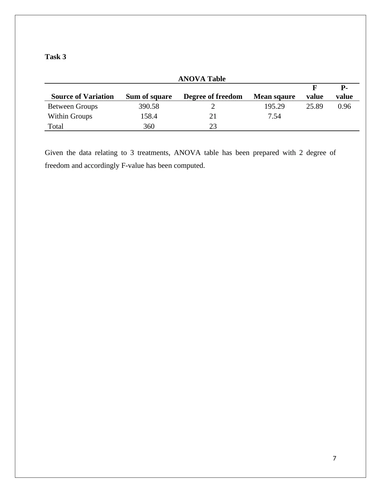
Given the data relating to 3 treatments, ANOVA table has been prepared with 2 degree of
freedom and accordingly F-value has been computed.
7

Task 4
(a)
Coefficients
Standar
d Error t Stat
Intercept 3.00 0.00
Variable
x 0.50 0.46 1.08
Variable
y 0.47 0.04 12.23
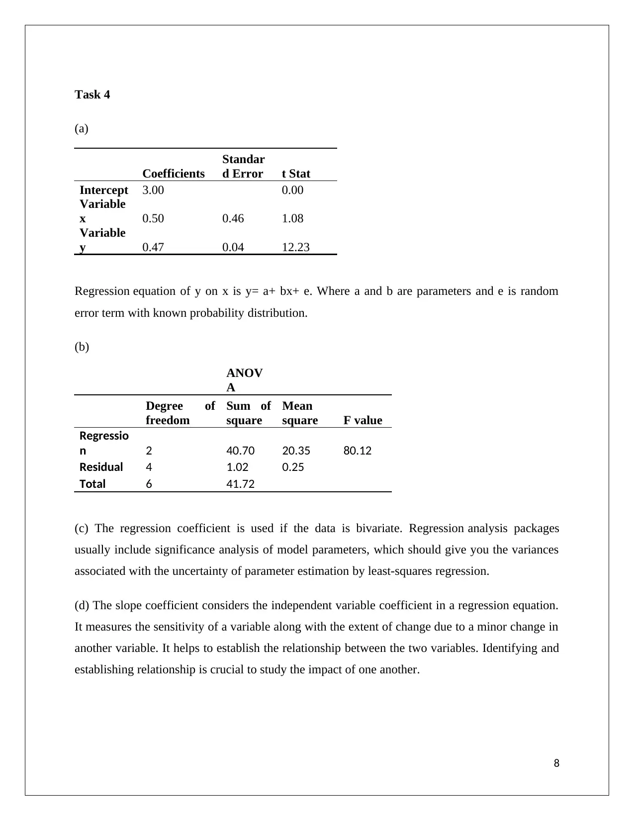
Regression equation of y on x is y= a+ bx+ e. Where a and b are parameters and e is random
error term with known probability distribution.
(b)
ANOV
A
Degree of
freedom
Sum of
square
Mean
square F value
Regressio
n 2 40.70 20.35 80.12
Residual 4 1.02 0.25
Total 6 41.72
(c) The regression coefficient is used if the data is bivariate. Regression analysis packages
usually include significance analysis of model parameters, which should give you the variances
associated with the uncertainty of parameter estimation by least-squares regression.
(d) The slope coefficient considers the independent variable coefficient in a regression equation.
It measures the sensitivity of a variable along with the extent of change due to a minor change in
another variable. It helps to establish the relationship between the two variables. Identifying and
establishing relationship is crucial to study the impact of one another.
8

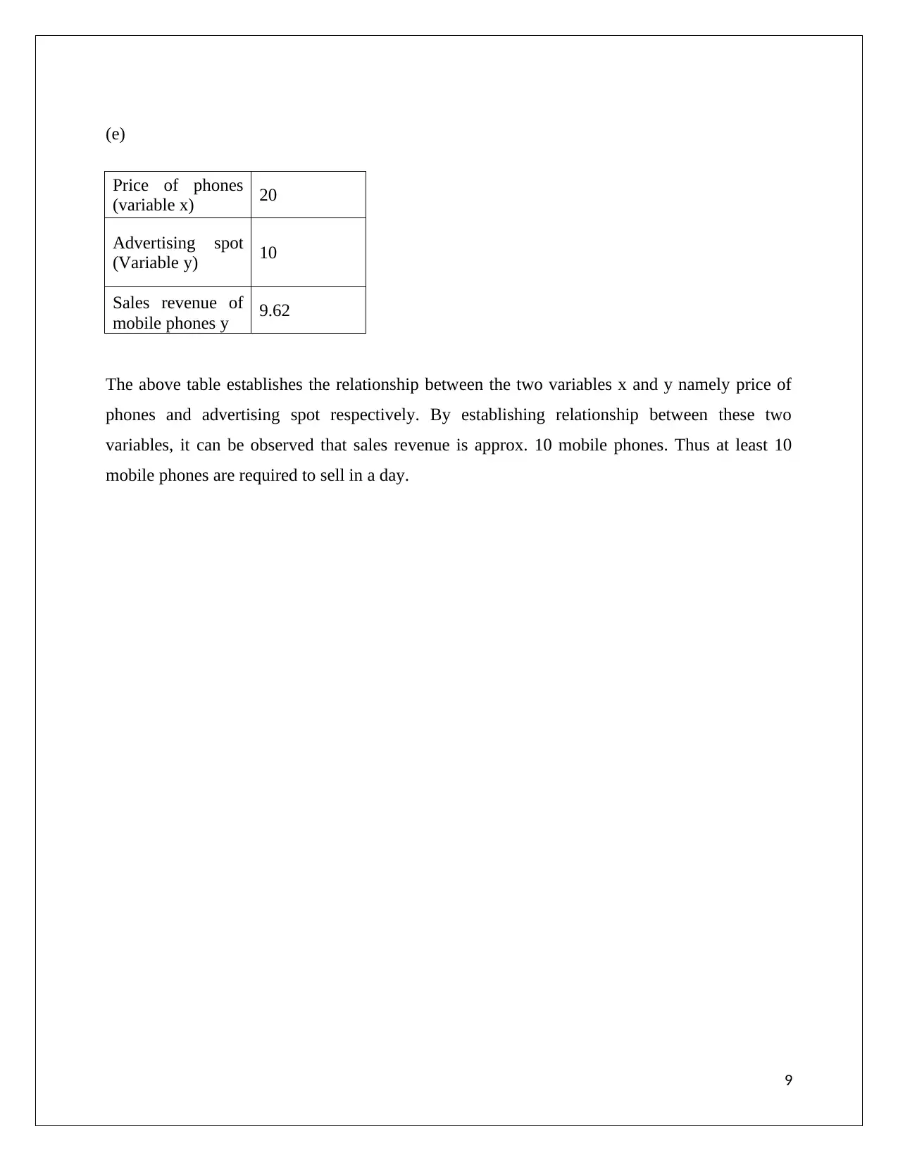
(e)
Price of phones
(variable x) 20
Advertising spot
(Variable y) 10
Sales revenue of
mobile phones y 9.62
The above table establishes the relationship between the two variables x and y namely price of
phones and advertising spot respectively. By establishing relationship between these two
variables, it can be observed that sales revenue is approx. 10 mobile phones. Thus at least 10
mobile phones are required to sell in a day.
9

Conclusion
From the discussion throughout the report it can be concluded and observed that the person
applying the tools and techniques should carefully apply it. Only then it can achieve the desired
result and can arrive at the correct decision. It is very important not to apply statistical tools and
techniques but also to correctly interpret and analyse the data. Otherwise it may bring wrong
conclusion and the reader can arrive at the wrong conclusion. For the better result, it is very
important and crucial to consider the limitations of the tools and techniques that have been
applied in the given tasks. This will facilitate the reader or user to get into the direction in which
the report is intended to.
10

References
 Barnes, E. A., & Barnes, R. J. 2015. Estimating linear trends: Simple linear regression versus
epoch differences. Journal of Climate, 28(24), 9969-9976.
 Elamir, E. A. 2015. Analysis of Mean Absolute Deviation for Randomized Block Design under
Laplace Distribution. American Journal of Theoretical and Applied Statistics, 4(3), 138-149.
 Figueiredo Filho, D. B., Paranhos, R., Rocha, E. C. D., Batista, M., Silva Jr, J. A. D., Santos, M.
L. W. D., & Marino, J. G. 2013. When is statistical significance not significant? Brazilian
Political Science Review, 7(1), 31-55.
 Frost, J., 2013. How to Interpret Regression Analysis Results: P-values and Coefficients. The
Minitab Blog. [Online]. Also available at http://blog.minitab.com/blog/adventures-in-statistics-
2/how-to-interpret-regression-analysis-results-p-values-and-coefficients
 Main, M. E., & Ogaz, V. L. 2016. Common Statistical Tests and Interpretation in Nursing
Research. International Journal of Faith Community Nursing, 2(3), 5.
 Nahas, J. J., 2012. Statistical Design of Experiments‐Part IV Analysis of Variance. University of
Notre dam. [Online]. Also available at https://www3.nd.edu/~jnahas/DoE_III_ANOVA_V2.pdf.
 Schneider, J. W. 2015. Null hypothesis significance tests. A mix-up of two different theories: the
basis for widespread confusion and numerous misinterpretations. Danish Centre for Studies in
Research and Research Policy, 102(1), 411-432.
 Winter, B. 2015. The F distribution and the basic principle behind ANOVAs. Tutorial. Also
available at http://www.bodowinter.com/tutorial/bw_anova_general.pdf.
11