Statistical Analysis and Data Interpretation

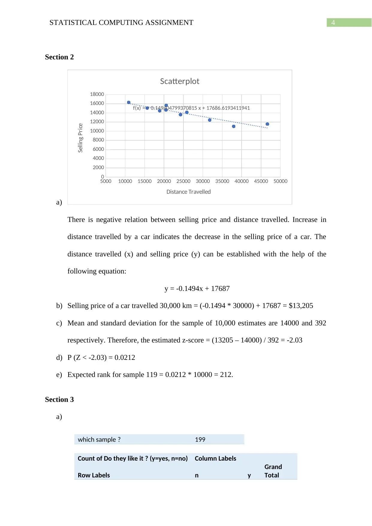
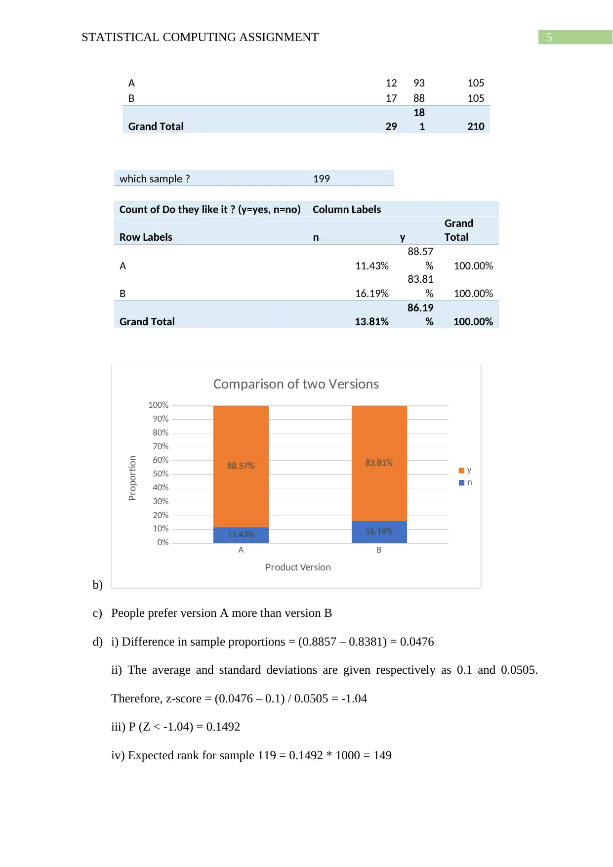
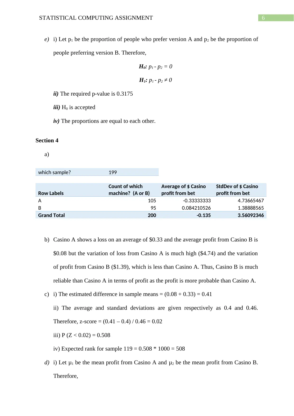
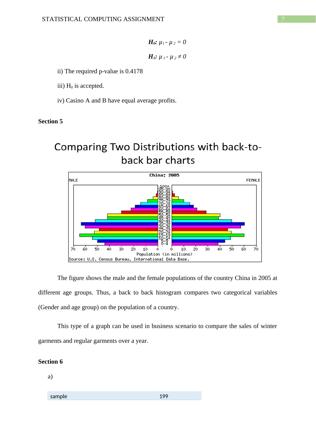
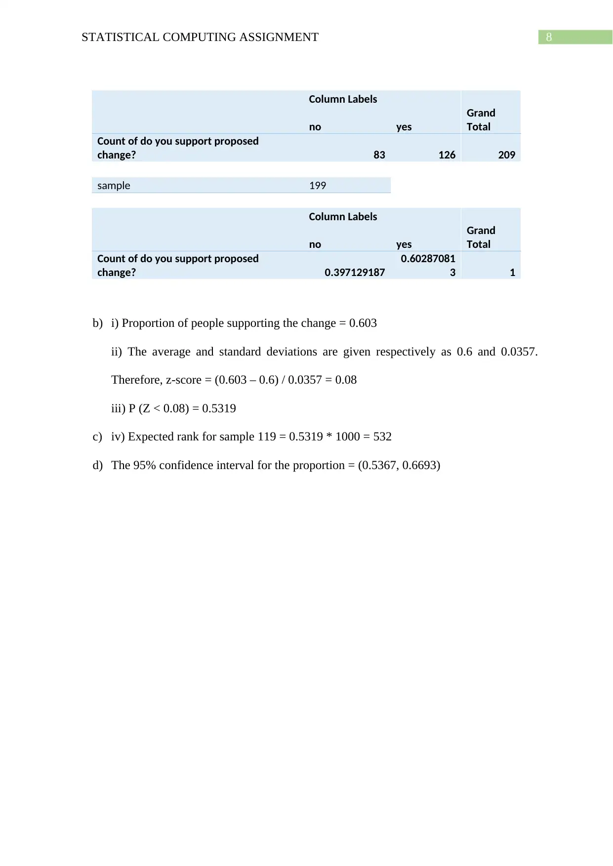
This assignment delves into various statistical concepts. Students are tasked with analyzing sample data from two casinos to determine if there's a significant difference in their average profits. They apply hypothesis testing, calculate confidence intervals, and interpret the results. Additionally, they analyze a demographic dataset of China's population in 2005, using a back-to-back histogram for comparison. Finally, students evaluate survey data on public support for a proposed change, calculating proportions and conducting a z-test.

Running Head: STATISTICAL COMPUTING ASSIGNMENT
Statistical Computing Assignment
Name of the Student
Name of the University
Author Note

1STATISTICAL COMPUTING ASSIGNMENT
Executive Summary
This assignment is mainly about understanding the methods which are used to compare two
types of variables. It can be between a qualitative and a quantitative variable, two qualitative
variables and two quantitative variables. To compare and assess the relationship between the
two dataset is necessary. Thus, the definition of dataset is discussed in the first section and
the relationship between the different types of variables are discussed in the sections that
follow using appropriate computational techniques.

2STATISTICAL COMPUTING ASSIGNMENT
Table of Contents
Section 1.....................................................................................................................................3
Section 2.....................................................................................................................................4
Section 3.....................................................................................................................................4
Section 4.....................................................................................................................................6
Section 5.....................................................................................................................................7
Section 6.....................................................................................................................................7

3STATISTICAL COMPUTING ASSIGNMENT
Section 1
Any type of information that can be collected about anything is known as data. To
illustrate, let an example be taken. In a school, the marks of physics, maths, statistics and the
gender of the students are recorded. All the marks and the gender are the information on each
of the students. All this information that has been collected is known as data. A file
containing all this information will be known as a dataset.
Now, this dataset contains information on the marks of students and the gender of the
students. Thus gender, marks on physics, maths and statistics will be known as variables.
Thus, it can be said that a variable contains values of a dataset and the values of the variables
changes from time to time. All the students will not secure the same marks and will not be of
the same gender. Thus, these are variables.
Now variables are of two types – Qualitative and Quantitative. Qualitative variables
contain values which describe certain characteristics of the variables. In this example, the
gender of the students is qualitative variable as it will indicate whether the student is a male
or a female. Quantitative variable is the type of variable which contains numerical values
about a variable. In this example, marks is a quantitative variable.
There are various ways to compare each of these variables. Two quantitative variables
can be compared and their relationship can be estimated with the help of a scatter diagram.
Two qualitative variables can be compared by calculating their proportion of occurrence. A
qualitative and a quantitative variable can be compared by evaluating the average of each of
the qualitative groups and comparing them.
These comparisons can be done very easily with the help of computing softwares. The
softwares reduce the labour and time. Thus, it is a very useful component for the purpose of
comparison and is widely used nowadays.

4STATISTICAL COMPUTING ASSIGNMENT
Section 2
a)
5000 10000 15000 20000 25000 30000 35000 40000 45000 50000
0
2000
4000
6000
8000
10000
12000
14000
16000
18000
f(x) = − 0.149404799370815 x + 17686.6193411941
Scatterplot
Distance Travelled
Selling Price
There is negative relation between selling price and distance travelled. Increase in
distance travelled by a car indicates the decrease in the selling price of a car. The
distance travelled (x) and selling price (y) can be established with the help of the
following equation:
y = -0.1494x + 17687
b) Selling price of a car travelled 30,000 km = (-0.1494 * 30000) + 17687 = $13,205
c) Mean and standard deviation for the sample of 10,000 estimates are 14000 and 392
respectively. Therefore, the estimated z-score = (13205 – 14000) / 392 = -2.03
d) P (Z < -2.03) = 0.0212
e) Expected rank for sample 119 = 0.0212 * 10000 = 212.
Section 3
a)
which sample ? 199
Count of Do they like it ? (y=yes, n=no) Column Labels
Row Labels n y
Grand
Total

5STATISTICAL COMPUTING ASSIGNMENT
A 12 93 105
B 17 88 105
Grand Total 29
18
1 210
which sample ? 199
Count of Do they like it ? (y=yes, n=no) Column Labels
Row Labels n y
Grand
Total
A 11.43%
88.57
% 100.00%
B 16.19%
83.81
% 100.00%
Grand Total 13.81%
86.19
% 100.00%
b)
A B
0%
10%
20%
30%
40%
50%
60%
70%
80%
90%
100%
11.43% 16.19%
88.57% 83.81%
Comparison of two Versions
y
n
Product Version
Proportion
c) People prefer version A more than version B
d) i) Difference in sample proportions = (0.8857 – 0.8381) = 0.0476
ii) The average and standard deviations are given respectively as 0.1 and 0.0505.
Therefore, z-score = (0.0476 – 0.1) / 0.0505 = -1.04
iii) P (Z < -1.04) = 0.1492
iv) Expected rank for sample 119 = 0.1492 * 1000 = 149

6STATISTICAL COMPUTING ASSIGNMENT
e) i) Let p1 be the proportion of people who prefer version A and p2 be the proportion of
people preferring version B. Therefore,
H0: p1 - p2 = 0
H1: p1 - p2 ≠ 0
ii) The required p-value is 0.3175
iii) H0 is accepted
iv) The proportions are equal to each other.
Section 4
a)
which sample? 199
Row Labels
Count of which
machine? (A or B)
Average of $ Casino
profit from bet
StdDev of $ Casino
profit from bet
A 105 -0.33333333 4.73665467
B 95 0.084210526 1.38888565
Grand Total 200 -0.135 3.56092346
b) Casino A shows a loss on an average of $0.33 and the average profit from Casino B is
$0.08 but the variation of loss from Casino A is much high ($4.74) and the variation
of profit from Casino B ($1.39), which is less than Casino A. Thus, Casino B is much
reliable than Casino A in terms of profit as the profit is more probable than Casino A.
c) i) The estimated difference in sample means = (0.08 + 0.33) = 0.41
ii) The average and standard deviations are given respectively as 0.4 and 0.46.
Therefore, z-score = (0.41 – 0.4) / 0.46 = 0.02
iii) P (Z < 0.02) = 0.508
iv) Expected rank for sample 119 = 0.508 * 1000 = 508
d) i) Let μ1 be the mean profit from Casino A and μ2 be the mean profit from Casino B.
Therefore,

7STATISTICAL COMPUTING ASSIGNMENT
H0: μ1 - μ 2 = 0
H1: μ 1 - μ 2 ≠ 0
ii) The required p-value is 0.4178
iii) H0 is accepted.
iv) Casino A and B have equal average profits.
Section 5
The figure shows the male and the female populations of the country China in 2005 at
different age groups. Thus, a back to back histogram compares two categorical variables
(Gender and age group) on the population of a country.
This type of a graph can be used in business scenario to compare the sales of winter
garments and regular garments over a year.
Section 6
a)
sample 199

8STATISTICAL COMPUTING ASSIGNMENT
Column Labels
no yes
Grand
Total
Count of do you support proposed
change? 83 126 209
sample 199
Column Labels
no yes
Grand
Total
Count of do you support proposed
change? 0.397129187
0.60287081
3 1
b) i) Proportion of people supporting the change = 0.603
ii) The average and standard deviations are given respectively as 0.6 and 0.0357.
Therefore, z-score = (0.603 – 0.6) / 0.0357 = 0.08
iii) P (Z < 0.08) = 0.5319
c) iv) Expected rank for sample 119 = 0.5319 * 1000 = 532
d) The 95% confidence interval for the proportion = (0.5367, 0.6693)