Regression Analysis for Education, Age Group, and Household Size

This assignment provides a comprehensive analysis of three different regression models: one for education (educ), another for age group (Agegp), and the last one for household size (hhsize). The results include source information, model statistics, residual analysis, R-squared values, and adjusted R-squared values. Each regression model has its own coefficients, standard errors, t-values, p-values, and confidence intervals for the variable 'IPV' (which is likely an indicator of some sort). The models also report the constant term (_cons) with its respective statistics. The summary provides a detailed overview of each regression analysis, including statistical measures such as root mean square error (RMSE), R-squared values, and adjusted R-squared values.

STATISTICAL METHODS IN
EPIDEMIOLOGY 2019

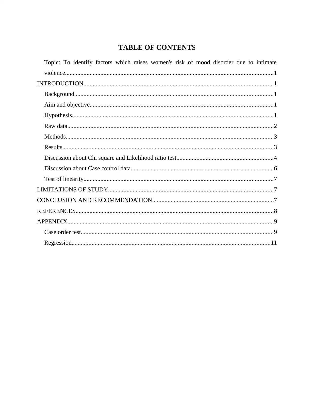
TABLE OF CONTENTS
Topic: To identify factors which raises women's risk of mood disorder due to intimate
violence.......................................................................................................................................1
INTRODUCTION...........................................................................................................................1
Background.................................................................................................................................1
Aim and objective.......................................................................................................................1
Hypothesis...................................................................................................................................1
Raw data......................................................................................................................................2
Methods.......................................................................................................................................3
Results.........................................................................................................................................3
Discussion about Chi square and Likelihood ratio test...............................................................4
Discussion about Case control data.............................................................................................6
Test of linearity...........................................................................................................................7
LIMITATIONS OF STUDY...........................................................................................................7
CONCLUSION AND RECOMMENDATION...............................................................................7
REFERENCES................................................................................................................................8
APPENDIX......................................................................................................................................9
Case order test.............................................................................................................................9
Regression.................................................................................................................................11

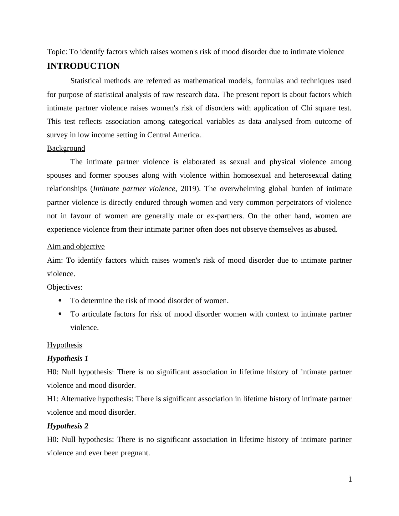
Topic: To identify factors which raises women's risk of mood disorder due to intimate violence
INTRODUCTION
Statistical methods are referred as mathematical models, formulas and techniques used
for purpose of statistical analysis of raw research data. The present report is about factors which
intimate partner violence raises women's risk of disorders with application of Chi square test.
This test reflects association among categorical variables as data analysed from outcome of
survey in low income setting in Central America.
Background
The intimate partner violence is elaborated as sexual and physical violence among
spouses and former spouses along with violence within homosexual and heterosexual dating
relationships (Intimate partner violence, 2019). The overwhelming global burden of intimate
partner violence is directly endured through women and very common perpetrators of violence
not in favour of women are generally male or ex-partners. On the other hand, women are
experience violence from their intimate partner often does not observe themselves as abused.
Aim and objective
Aim: To identify factors which raises women's risk of mood disorder due to intimate partner
violence.
Objectives:
 To determine the risk of mood disorder of women.
 To articulate factors for risk of mood disorder women with context to intimate partner
violence.
Hypothesis
Hypothesis 1
H0: Null hypothesis: There is no significant association in lifetime history of intimate partner
violence and mood disorder.
H1: Alternative hypothesis: There is significant association in lifetime history of intimate partner
violence and mood disorder.
Hypothesis 2
H0: Null hypothesis: There is no significant association in lifetime history of intimate partner
violence and ever been pregnant.
1

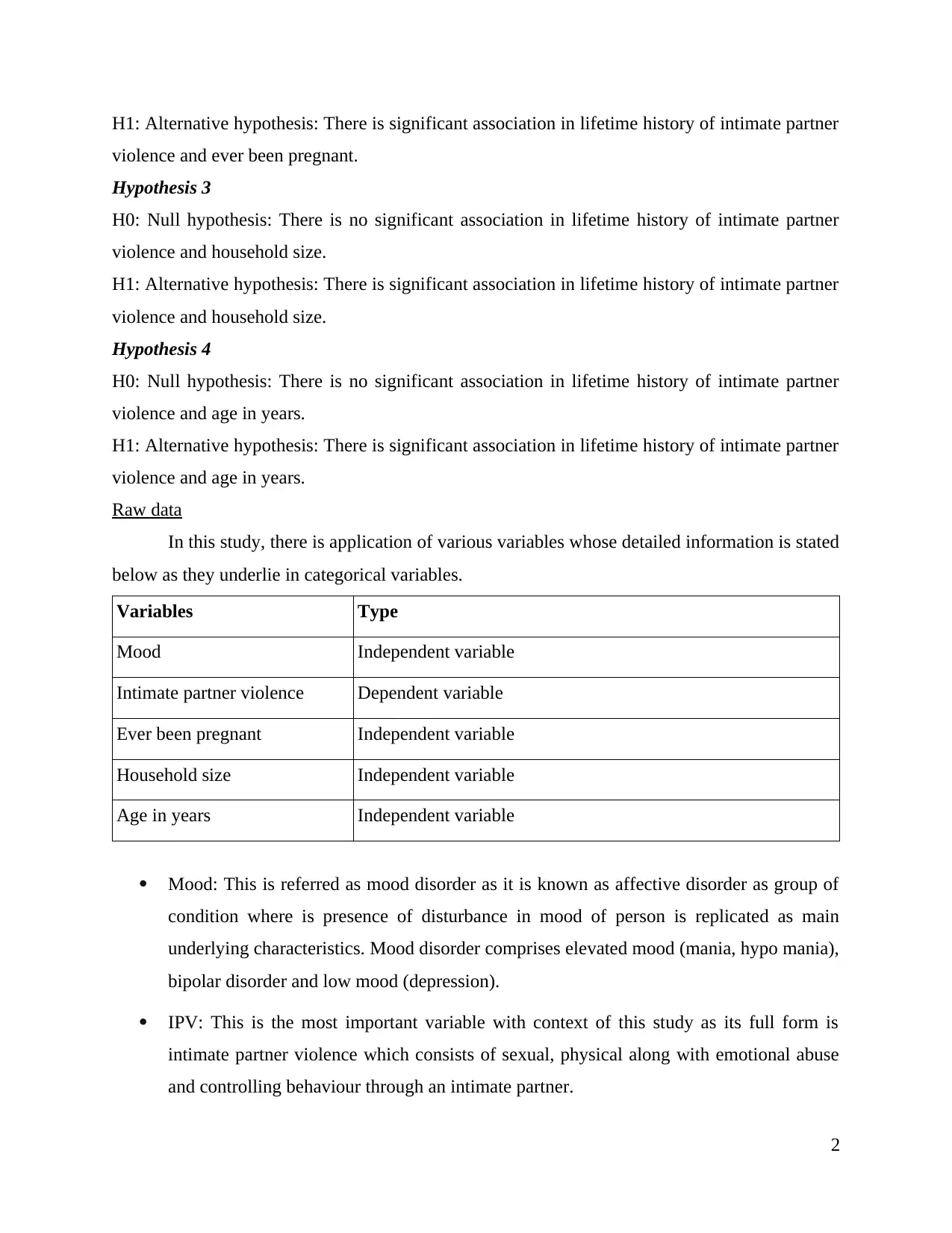
H1: Alternative hypothesis: There is significant association in lifetime history of intimate partner
violence and ever been pregnant.
Hypothesis 3
H0: Null hypothesis: There is no significant association in lifetime history of intimate partner
violence and household size.
H1: Alternative hypothesis: There is significant association in lifetime history of intimate partner
violence and household size.
Hypothesis 4
H0: Null hypothesis: There is no significant association in lifetime history of intimate partner
violence and age in years.
H1: Alternative hypothesis: There is significant association in lifetime history of intimate partner
violence and age in years.
Raw data
In this study, there is application of various variables whose detailed information is stated
below as they underlie in categorical variables.
Variables Type
Mood Independent variable
Intimate partner violence Dependent variable
Ever been pregnant Independent variable
Household size Independent variable
Age in years Independent variable
 Mood: This is referred as mood disorder as it is known as affective disorder as group of
condition where is presence of disturbance in mood of person is replicated as main
underlying characteristics. Mood disorder comprises elevated mood (mania, hypo mania),
bipolar disorder and low mood (depression).
 IPV: This is the most important variable with context of this study as its full form is
intimate partner violence which consists of sexual, physical along with emotional abuse
and controlling behaviour through an intimate partner.
2

 Everpreg: This variable is reflects the women who had ever been pregnant or not.
 Hhsize: In this variable, size of household has been described with categories such as 1-3,
4-5, 6-9, 10+.
 Agegp: This variable is referred as age in years which is grouped in 5 categories which
are 18 to 24, 25 to 29, 30 to 34, 35 to 39 and 40 to 50 years.
Methods
The data has been analysed on basis of identifying that intimate partner's violence raises
women's risk of mood disorders with large cross sectional survey conducted in low income
setting in Central America whose aim was to investigate about factors association with risk of
mood disorders in women. It is referred as secondary source of collecting data. For purpose of
extracting association among dependent and independent variable there is application of Mantel
Hanzel test, test of departure from linearity, confounding for case orders, Chi-squared test and
likelihood ratio.
Results
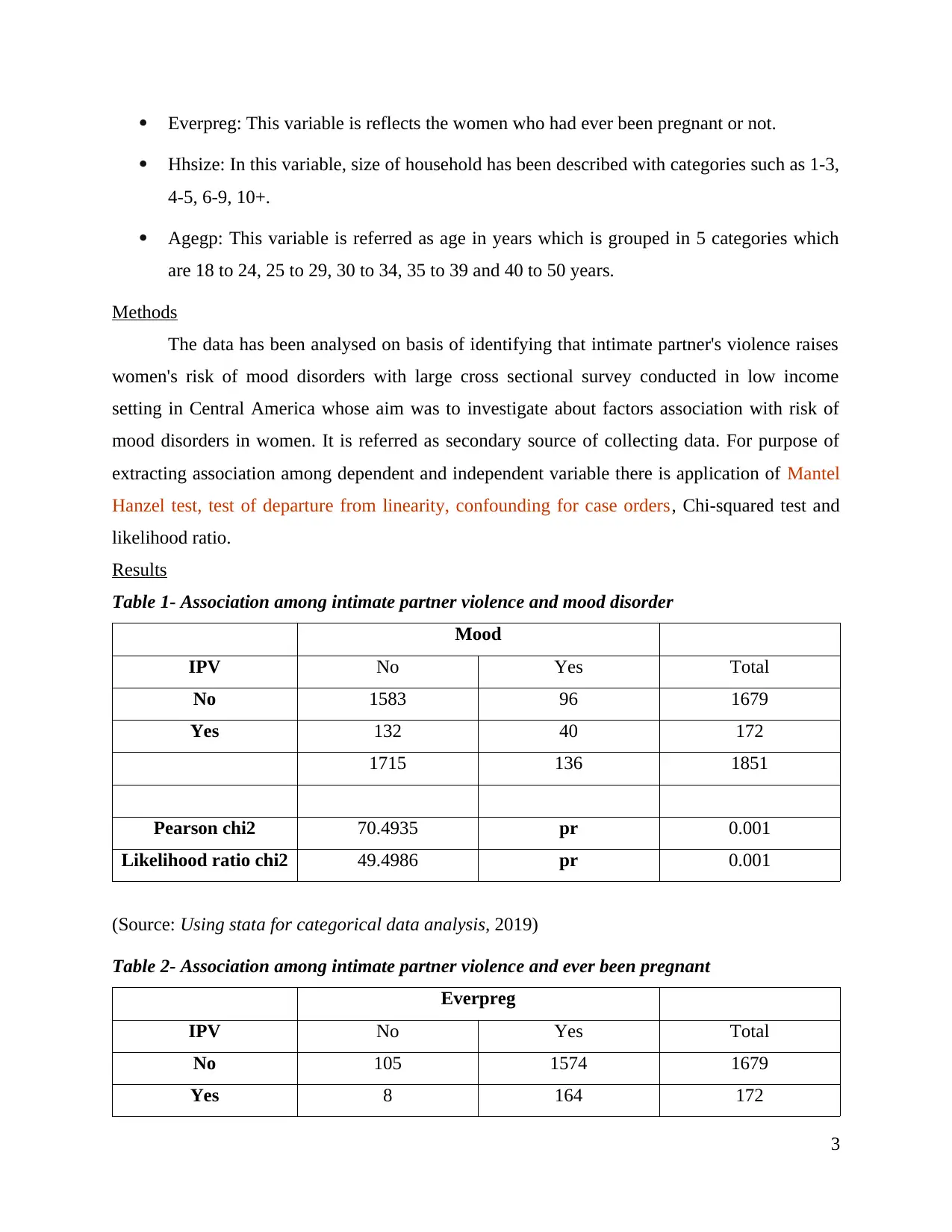
Table 1- Association among intimate partner violence and mood disorder
Mood
IPV No Yes Total
No 1583 96 1679
Yes 132 40 172
1715 136 1851
Pearson chi2 70.4935 pr 0.001
Likelihood ratio chi2 49.4986 pr 0.001
(Source: Using stata for categorical data analysis, 2019)
Table 2- Association among intimate partner violence and ever been pregnant
Everpreg
IPV No Yes Total
No 105 1574 1679
Yes 8 164 172
3

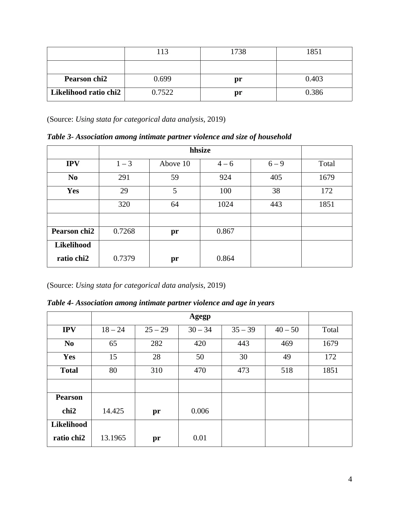
113 1738 1851
Pearson chi2 0.699 pr 0.403
Likelihood ratio chi2 0.7522 pr 0.386
(Source: Using stata for categorical data analysis, 2019)
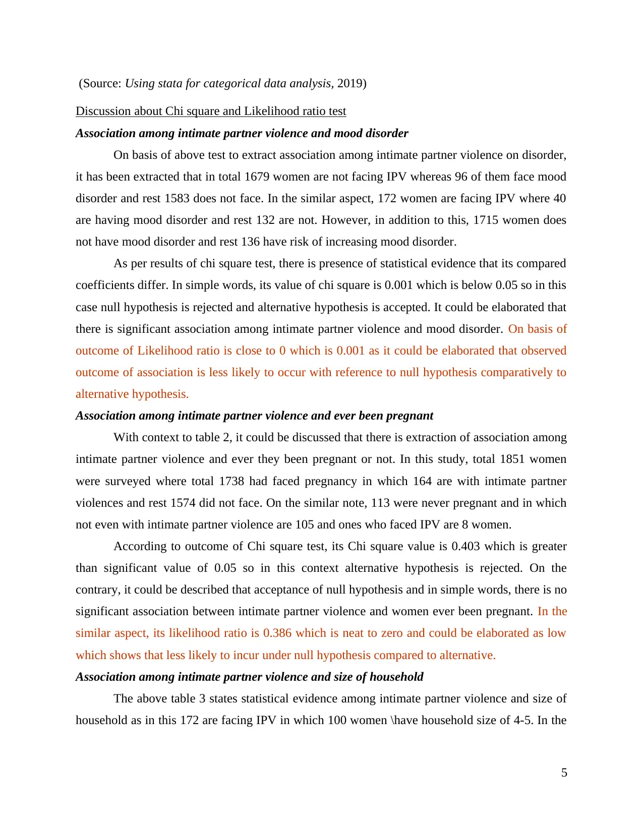
Table 3- Association among intimate partner violence and size of household
hhsize
IPV 1 – 3 Above 10 4 – 6 6 – 9 Total
No 291 59 924 405 1679
Yes 29 5 100 38 172
320 64 1024 443 1851
Pearson chi2 0.7268 pr 0.867
Likelihood
ratio chi2 0.7379 pr 0.864
(Source: Using stata for categorical data analysis, 2019)
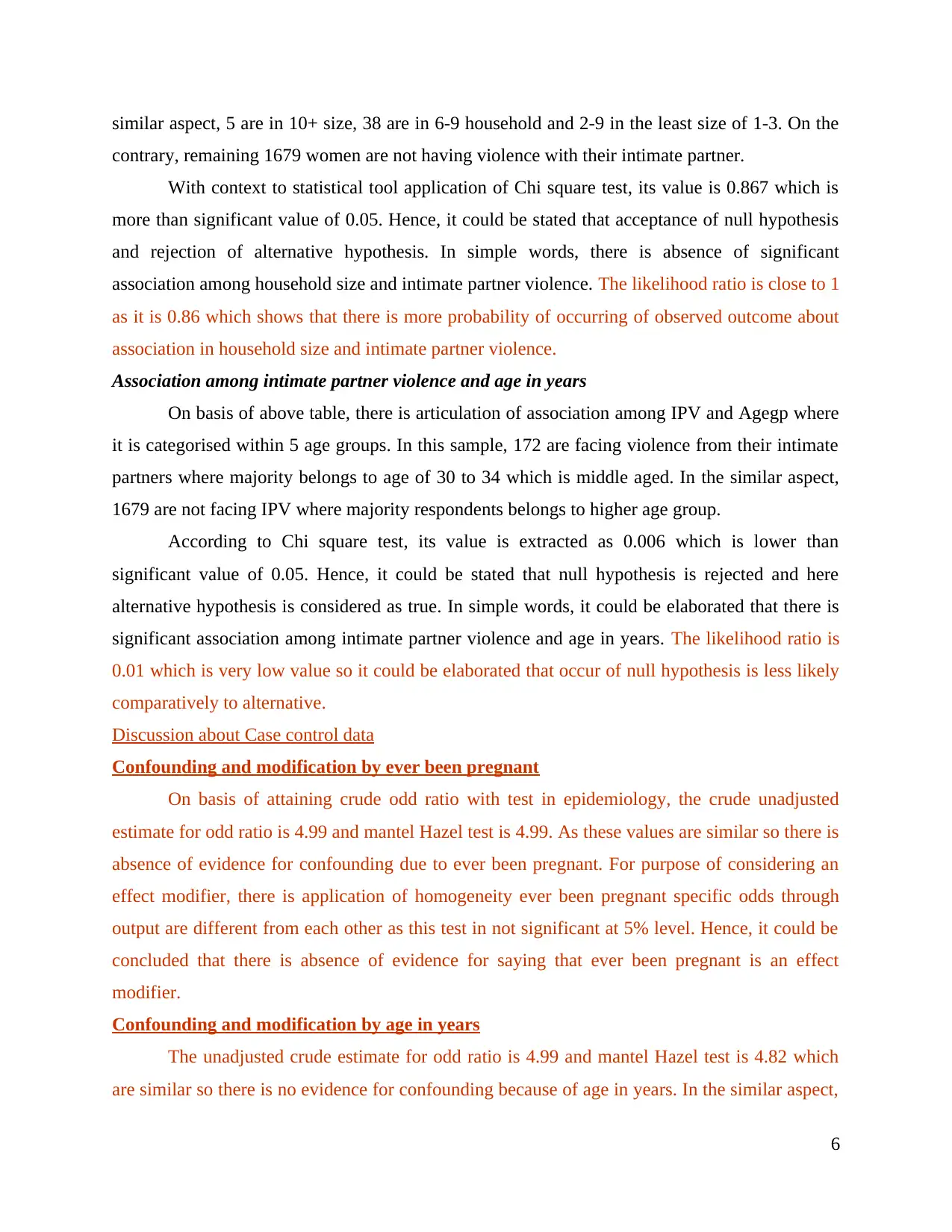
Table 4- Association among intimate partner violence and age in years
Agegp
IPV 18 – 24 25 – 29 30 – 34 35 – 39 40 – 50 Total
No 65 282 420 443 469 1679
Yes 15 28 50 30 49 172
Total 80 310 470 473 518 1851
Pearson
chi2 14.425 pr 0.006
Likelihood
ratio chi2 13.1965 pr 0.01
4

(Source: Using stata for categorical data analysis, 2019)
Discussion about Chi square and Likelihood ratio test
Association among intimate partner violence and mood disorder
On basis of above test to extract association among intimate partner violence on disorder,
it has been extracted that in total 1679 women are not facing IPV whereas 96 of them face mood
disorder and rest 1583 does not face. In the similar aspect, 172 women are facing IPV where 40
are having mood disorder and rest 132 are not. However, in addition to this, 1715 women does
not have mood disorder and rest 136 have risk of increasing mood disorder.
As per results of chi square test, there is presence of statistical evidence that its compared
coefficients differ. In simple words, its value of chi square is 0.001 which is below 0.05 so in this
case null hypothesis is rejected and alternative hypothesis is accepted. It could be elaborated that
there is significant association among intimate partner violence and mood disorder. On basis of
outcome of Likelihood ratio is close to 0 which is 0.001 as it could be elaborated that observed
outcome of association is less likely to occur with reference to null hypothesis comparatively to
alternative hypothesis.
Association among intimate partner violence and ever been pregnant
With context to table 2, it could be discussed that there is extraction of association among
intimate partner violence and ever they been pregnant or not. In this study, total 1851 women
were surveyed where total 1738 had faced pregnancy in which 164 are with intimate partner
violences and rest 1574 did not face. On the similar note, 113 were never pregnant and in which
not even with intimate partner violence are 105 and ones who faced IPV are 8 women.
According to outcome of Chi square test, its Chi square value is 0.403 which is greater
than significant value of 0.05 so in this context alternative hypothesis is rejected. On the
contrary, it could be described that acceptance of null hypothesis and in simple words, there is no
significant association between intimate partner violence and women ever been pregnant. In the
similar aspect, its likelihood ratio is 0.386 which is neat to zero and could be elaborated as low
which shows that less likely to incur under null hypothesis compared to alternative.
Association among intimate partner violence and size of household
The above table 3 states statistical evidence among intimate partner violence and size of
household as in this 172 are facing IPV in which 100 women \have household size of 4-5. In the
5

similar aspect, 5 are in 10+ size, 38 are in 6-9 household and 2-9 in the least size of 1-3. On the
contrary, remaining 1679 women are not having violence with their intimate partner.
With context to statistical tool application of Chi square test, its value is 0.867 which is
more than significant value of 0.05. Hence, it could be stated that acceptance of null hypothesis
and rejection of alternative hypothesis. In simple words, there is absence of significant
association among household size and intimate partner violence. The likelihood ratio is close to 1
as it is 0.86 which shows that there is more probability of occurring of observed outcome about
association in household size and intimate partner violence.
Association among intimate partner violence and age in years
On basis of above table, there is articulation of association among IPV and Agegp where
it is categorised within 5 age groups. In this sample, 172 are facing violence from their intimate
partners where majority belongs to age of 30 to 34 which is middle aged. In the similar aspect,
1679 are not facing IPV where majority respondents belongs to higher age group.
According to Chi square test, its value is extracted as 0.006 which is lower than
significant value of 0.05. Hence, it could be stated that null hypothesis is rejected and here
alternative hypothesis is considered as true. In simple words, it could be elaborated that there is
significant association among intimate partner violence and age in years. The likelihood ratio is
0.01 which is very low value so it could be elaborated that occur of null hypothesis is less likely
comparatively to alternative.
Discussion about Case control data
Confounding and modification by ever been pregnant
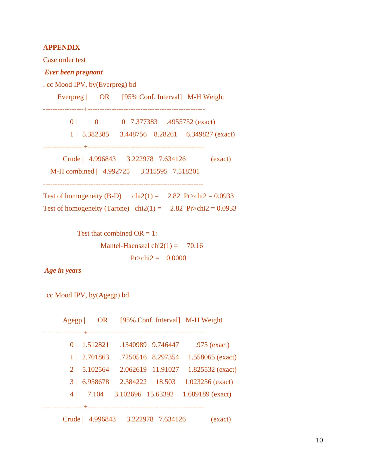
On basis of attaining crude odd ratio with test in epidemiology, the crude unadjusted
estimate for odd ratio is 4.99 and mantel Hazel test is 4.99. As these values are similar so there is
absence of evidence for confounding due to ever been pregnant. For purpose of considering an
effect modifier, there is application of homogeneity ever been pregnant specific odds through
output are different from each other as this test in not significant at 5% level. Hence, it could be
concluded that there is absence of evidence for saying that ever been pregnant is an effect
modifier.
Confounding and modification by age in years
The unadjusted crude estimate for odd ratio is 4.99 and mantel Hazel test is 4.82 which
are similar so there is no evidence for confounding because of age in years. In the similar aspect,
6

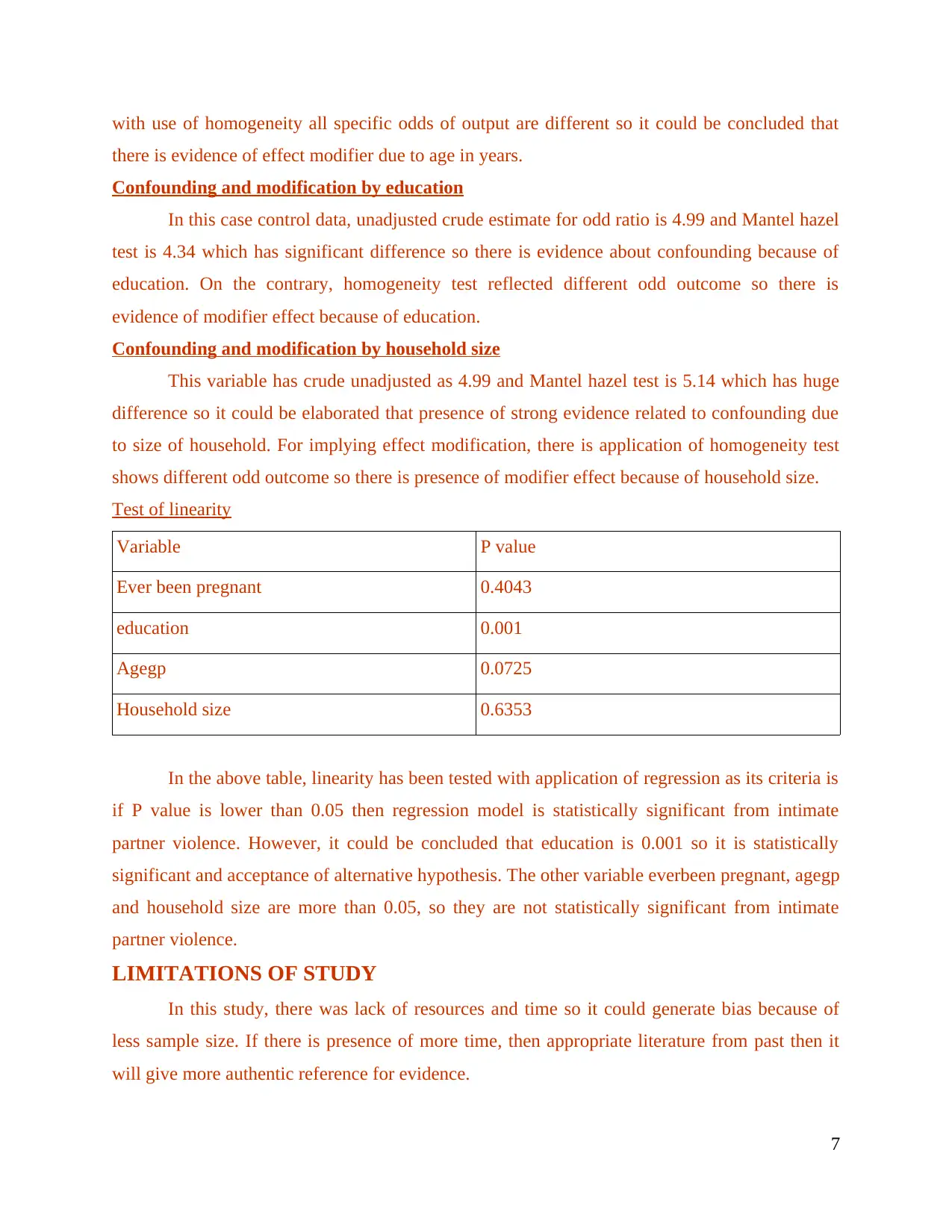
with use of homogeneity all specific odds of output are different so it could be concluded that
there is evidence of effect modifier due to age in years.
Confounding and modification by education
In this case control data, unadjusted crude estimate for odd ratio is 4.99 and Mantel hazel
test is 4.34 which has significant difference so there is evidence about confounding because of
education. On the contrary, homogeneity test reflected different odd outcome so there is
evidence of modifier effect because of education.
Confounding and modification by household size
This variable has crude unadjusted as 4.99 and Mantel hazel test is 5.14 which has huge
difference so it could be elaborated that presence of strong evidence related to confounding due
to size of household. For implying effect modification, there is application of homogeneity test
shows different odd outcome so there is presence of modifier effect because of household size.
Test of linearity
Variable P value
Ever been pregnant 0.4043
education 0.001
Agegp 0.0725
Household size 0.6353
In the above table, linearity has been tested with application of regression as its criteria is
if P value is lower than 0.05 then regression model is statistically significant from intimate
partner violence. However, it could be concluded that education is 0.001 so it is statistically
significant and acceptance of alternative hypothesis. The other variable everbeen pregnant, agegp
and household size are more than 0.05, so they are not statistically significant from intimate
partner violence.
LIMITATIONS OF STUDY
In this study, there was lack of resources and time so it could generate bias because of
less sample size. If there is presence of more time, then appropriate literature from past then it
will give more authentic reference for evidence.
7

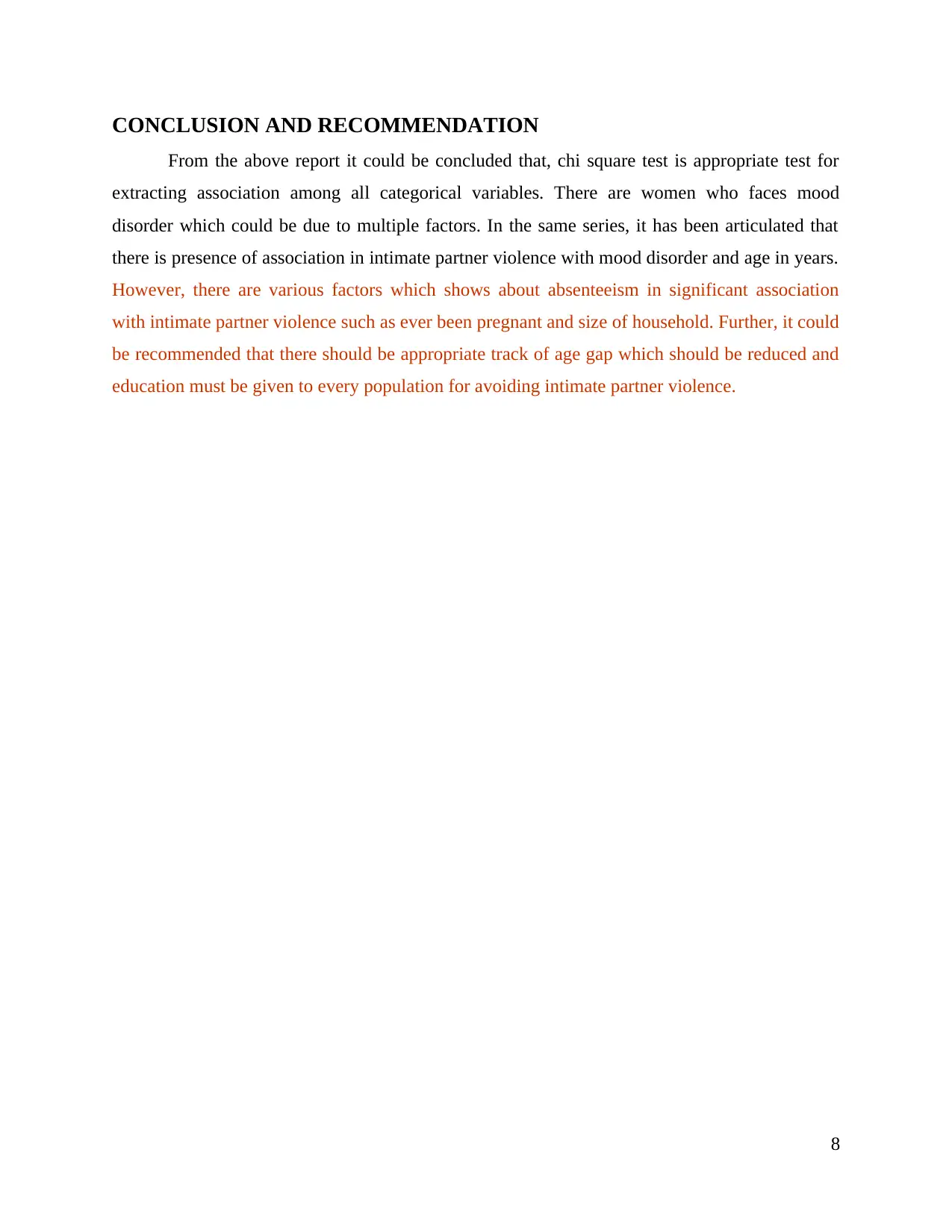
CONCLUSION AND RECOMMENDATION
From the above report it could be concluded that, chi square test is appropriate test for
extracting association among all categorical variables. There are women who faces mood
disorder which could be due to multiple factors. In the same series, it has been articulated that
there is presence of association in intimate partner violence with mood disorder and age in years.
However, there are various factors which shows about absenteeism in significant association
with intimate partner violence such as ever been pregnant and size of household. Further, it could
be recommended that there should be appropriate track of age gap which should be reduced and
education must be given to every population for avoiding intimate partner violence.
8

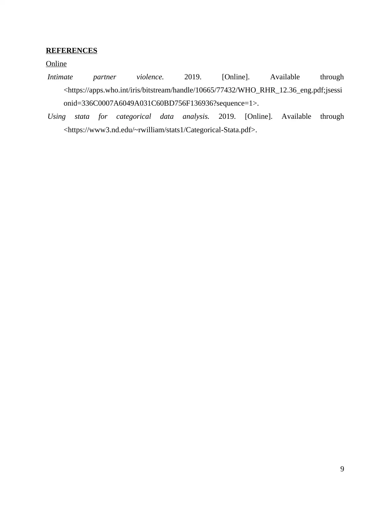
REFERENCES
Online
Intimate partner violence. 2019. [Online]. Available through
<https://apps.who.int/iris/bitstream/handle/10665/77432/WHO_RHR_12.36_eng.pdf;jsessi
onid=336C0007A6049A031C60BD756F136936?sequence=1>.
Using stata for categorical data analysis. 2019. [Online]. Available through
<https://www3.nd.edu/~rwilliam/stats1/Categorical-Stata.pdf>.
9

APPENDIX
Case order test
Ever been pregnant
. cc Mood IPV, by(Everpreg) bd
Everpreg | OR [95% Conf. Interval] M-H Weight
-----------------+-------------------------------------------------
0 | 0 0 7.377383 .4955752 (exact)
1 | 5.382385 3.448756 8.28261 6.349827 (exact)
-----------------+-------------------------------------------------
Crude | 4.996843 3.222978 7.634126 (exact)
M-H combined | 4.992725 3.315595 7.518201
-------------------------------------------------------------------
Test of homogeneity (B-D) chi2(1) = 2.82 Pr>chi2 = 0.0933
Test of homogeneity (Tarone) chi2(1) = 2.82 Pr>chi2 = 0.0933
Test that combined OR = 1:
Mantel-Haenszel chi2(1) = 70.16
Pr>chi2 = 0.0000
Age in years
. cc Mood IPV, by(Agegp) bd
Agegp | OR [95% Conf. Interval] M-H Weight
-----------------+-------------------------------------------------
0 | 1.512821 .1340989 9.746447 .975 (exact)
1 | 2.701863 .7250516 8.297354 1.558065 (exact)
2 | 5.102564 2.062619 11.91027 1.825532 (exact)
3 | 6.958678 2.384222 18.503 1.023256 (exact)
4 | 7.104 3.102696 15.63392 1.689189 (exact)
-----------------+-------------------------------------------------
Crude | 4.996843 3.222978 7.634126 (exact)
10

M-H combined | 4.825326 3.19878 7.278954
-------------------------------------------------------------------
Test of homogeneity (M-H) chi2(4) = 4.59 Pr>chi2 = 0.3315
Test of homogeneity (B-D) chi2(4) = 4.76 Pr>chi2 = 0.3123
Test that combined OR = 1:
Mantel-Haenszel chi2(1) = 67.97
Pr>chi2 = 0.0000
Education
. cc Mood IPV, by(educ) bd
educ | OR [95% Conf. Interval] M-H Weight
-----------------+-------------------------------------------------
0 | 4.875 1.907779 12.13083 1.981651 (exact)
1 | 4.238009 2.26876 7.683497 4.112903 (exact)
3 | 3.889655 1.244892 10.25907 1.40266 (exact)
-----------------+-------------------------------------------------
Crude | 4.996843 3.222978 7.634126 (exact)
M-H combined | 4.341204 2.852191 6.60757
-------------------------------------------------------------------
Test of homogeneity (M-H) chi2(2) = 0.13 Pr>chi2 = 0.9354
Test of homogeneity (B-D) chi2(2) = 0.13 Pr>chi2 = 0.9354
Test that combined OR = 1:
Mantel-Haenszel chi2(1) = 53.16
Pr>chi2 = 0.0000
Household size
. cc Mood IPV, by(hhsize) bd
hhsize | OR [95% Conf. Interval] M-H Weight
-----------------+-------------------------------------------------
11

0 | 5.453634 1.825895 14.93674 1.246875 (exact)
1 | 4.287805 2.224731 7.954806 3.603516 (exact)
2 | 7.291667 3.124158 16.39636 1.625282 (exact)
3 | 0 0 26.38884 .15625 (exact)
-----------------+-------------------------------------------------
Crude | 4.996843 3.222978 7.634126 (exact)
M-H combined | 5.142127 3.403759 7.768314
-------------------------------------------------------------------
Test of homogeneity (B-D) chi2(3) = 2.07 Pr>chi2 = 0.5578
Test of homogeneity (Tarone) chi2(3) = 2.07 Pr>chi2 = 0.5578
Test that combined OR = 1:
Mantel-Haenszel chi2(1) = 71.76
Pr>chi2 = 0.0000
Regression
Ever been pregnant
. regress Everpreg IPV
Source | SS df MS Number of obs = 1851
-------------+------------------------------ F( 1, 1849) = 0.70
Model | .04006832 1 .04006832 Prob > F = 0.4034
Residual | 106.061498 1849 .057361546 R-squared = 0.0004
-------------+------------------------------ Adj R-squared = -0.0002
Total | 106.101567 1850 .057352198 Root MSE = .2395
------------------------------------------------------------------------------
Everpreg | Coef. Std. Err. t P>|t| [95% Conf. Interval]
-------------+----------------------------------------------------------------
IPV | .0160256 .0191745 0.84 0.403 -.0215804 .0536315
_cons | .9374628 .005845 160.39 0.000 .9259993 .9489263
12

Education
. regress educ IPV
Source | SS df MS Number of obs = 1851
-------------+------------------------------ F( 1, 1849) = 33.17
Model | 42.5080771 1 42.5080771 Prob > F = 0.0000
Residual | 2369.44762 1849 1.28147519 R-squared = 0.0176
-------------+------------------------------ Adj R-squared = 0.0171
Total | 2411.9557 1850 1.30375984 Root MSE = 1.132
------------------------------------------------------------------------------
educ | Coef. Std. Err. t P>|t| [95% Conf. Interval]
-------------+----------------------------------------------------------------
IPV | -.5219746 .0906293 -5.76 0.000 -.6997212 -.344228
_cons | 1.8243 .0276267 66.03 0.000 1.770117 1.878483
------------------------------------------------------------------------------
Age in years
. regress Agegp IPV
Source | SS df MS Number of obs = 1851
-------------+------------------------------ F( 1, 1849) = 3.23
Model | 4.51699272 1 4.51699272 Prob > F = 0.0725
Residual | 2587.27339 1849 1.39928253 R-squared = 0.0017
-------------+------------------------------ Adj R-squared = 0.0012
Total | 2591.79038 1850 1.40096777 Root MSE = 1.1829
------------------------------------------------------------------------------
Agegp | Coef. Std. Err. t P>|t| [95% Conf. Interval]
-------------+----------------------------------------------------------------
IPV | -.1701525 .0947036 -1.80 0.073 -.3558897 .0155847
_cons | 2.577129 .0288687 89.27 0.000 2.520511 2.633748
13

------------------------------------------------------------------------------
Household size
. regress hhsize IPV
Source | SS df MS Number of obs = 1851
-------------+------------------------------ F( 1, 1849) = 0.22
Model | .11981745 1 .11981745 Prob > F = 0.6353
Residual | 984.843986 1849 .532636012 R-squared = 0.0001
-------------+------------------------------ Adj R-squared = -0.0004
Total | 984.963803 1850 .532412867 Root MSE = .72982
------------------------------------------------------------------------------
hhsize | Coef. Std. Err. t P>|t| [95% Conf. Interval]
-------------+----------------------------------------------------------------
IPV | -.0277124 .0584291 -0.47 0.635 -.1423062 .0868815
_cons | 1.138177 .0178111 63.90 0.000 1.103246 1.173109
14