Statistical Practice: One-sample t-test, Two-sample t-test in R

This document provides a comprehensive guide on statistical practice, focusing on one-sample t-test and two-sample t-test in R. It includes step-by-step instructions, output, and interpretation of the tests. The document also covers the assumptions of normality and provides appropriate plots to test them. Study material and solved assignments on statistical practice are available at Desklib.

STATISTICAL
PRACTICE

1. One-sample t-test in R
(a) First examine the distribution of the total seconds by doing the following:
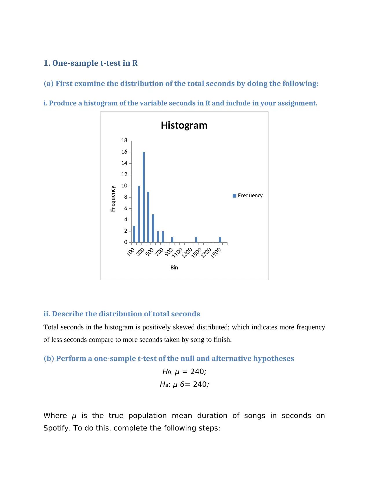
i. Produce a histogram of the variable seconds in R and include in your assignment.
100
300
500
700
900
1100
1300
1500
1700
1900
0
2
4
6
8
10
12
14
16
18
Histogram
Frequency
Bin
Frequency
ii. Describe the distribution of total seconds
Total seconds in the histogram is positively skewed distributed; which indicates more frequency
of less seconds compare to more seconds taken by song to finish.
(b) Perform a one-sample t-test of the null and alternative hypotheses
H0: μ = 240;
Ha: μ 6= 240;
Where μ is the true population mean duration of songs in seconds on
Spotify. To do this, complete the following steps:

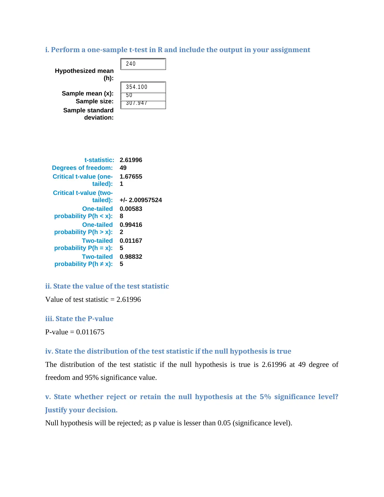
i. Perform a one-sample t-test in R and include the output in your assignment
Hypothesized mean
(h):
Sample mean (x):
Sample size:
Sample standard
deviation:
t-statistic: 2.61996
Degrees of freedom: 49
Critical t-value (one-
tailed):
1.67655
1
Critical t-value (two-
tailed): +/- 2.00957524
One-tailed
probability P(h < x):
0.00583
8
One-tailed
probability P(h > x):
0.99416
2
Two-tailed
probability P(h = x):
0.01167
5
Two-tailed
probability P(h ≠ x):
0.98832
5
ii. State the value of the test statistic
Value of test statistic = 2.61996
iii. State the P-value
P-value = 0.011675
iv. State the distribution of the test statistic if the null hypothesis is true
The distribution of the test statistic if the null hypothesis is true is 2.61996 at 49 degree of
freedom and 95% significance value.
v. State whether reject or retain the null hypothesis at the 5% significance level?
Justify your decision.
Null hypothesis will be rejected; as p value is lesser than 0.05 (significance level).
3 0 7 . 9 4 7
5 0
3 5 4 . 1 0 0
2 4 0

(c) Using your R output, calculate a 95% confidence interval for the mean song
duration in seconds. Interpret this interval in context.
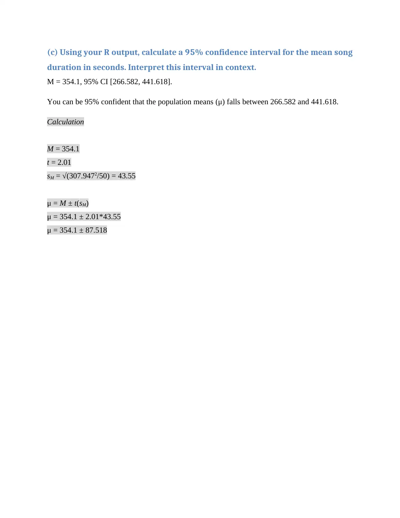
M = 354.1, 95% CI [266.582, 441.618].
You can be 95% confident that the population means (μ) falls between 266.582 and 441.618.
Calculation
M = 354.1
t = 2.01
sM = √(307.9472/50) = 43.55
μ = M ± t(sM)
μ = 354.1 ± 2.01*43.55
μ = 354.1 ± 87.518

(d) Check the assumption of normality of the sample mean with the following
steps:
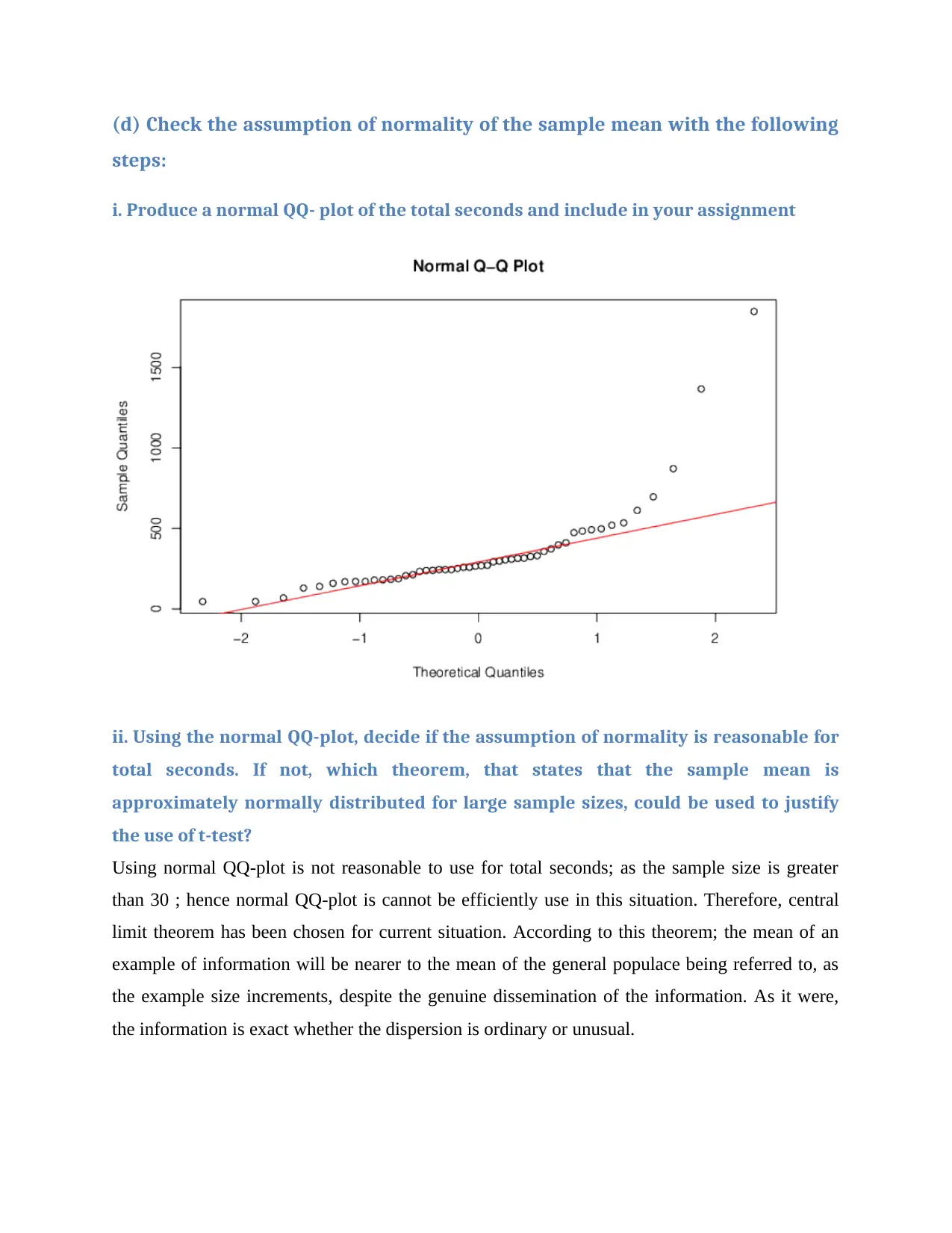
i. Produce a normal QQ- plot of the total seconds and include in your assignment
ii. Using the normal QQ-plot, decide if the assumption of normality is reasonable for
total seconds. If not, which theorem, that states that the sample mean is
approximately normally distributed for large sample sizes, could be used to justify
the use of t-test?
Using normal QQ-plot is not reasonable to use for total seconds; as the sample size is greater
than 30 ; hence normal QQ-plot is cannot be efficiently use in this situation. Therefore, central
limit theorem has been chosen for current situation. According to this theorem; the mean of an
example of information will be nearer to the mean of the general populace being referred to, as
the example size increments, despite the genuine dissemination of the information. As it were,
the information is exact whether the dispersion is ordinary or unusual.

2. Two-sample T-test in R
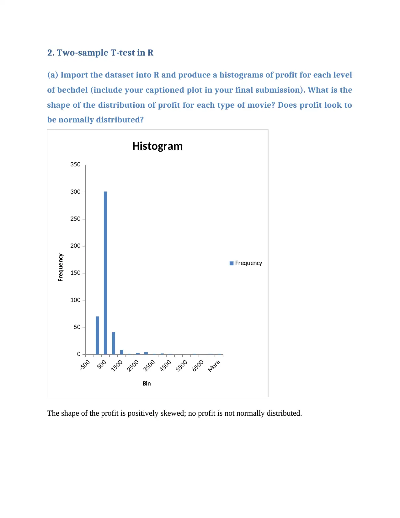
(a) Import the dataset into R and produce a histograms of profit for each level
of bechdel (include your captioned plot in your final submission). What is the
shape of the distribution of profit for each type of movie? Does profit look to
be normally distributed?
-500
500
1500
2500
3500
4500
5500
6500
More
0
50
100
150
200
250
300
350
Histogram
Frequency
Bin
Frequency
The shape of the profit is positively skewed; no profit is not normally distributed.

(b) Perform a two-sample t-test in R.
i. Write down appropriate null and alternative hypotheses for the two-sample t-test.
Remember to define any parameters used.
Null Hypotheses H0: There’s no significance difference between result of Bechdel and Profit
Alternative Hypotheses H1: There’s significance difference between result of Bechdel and profit.
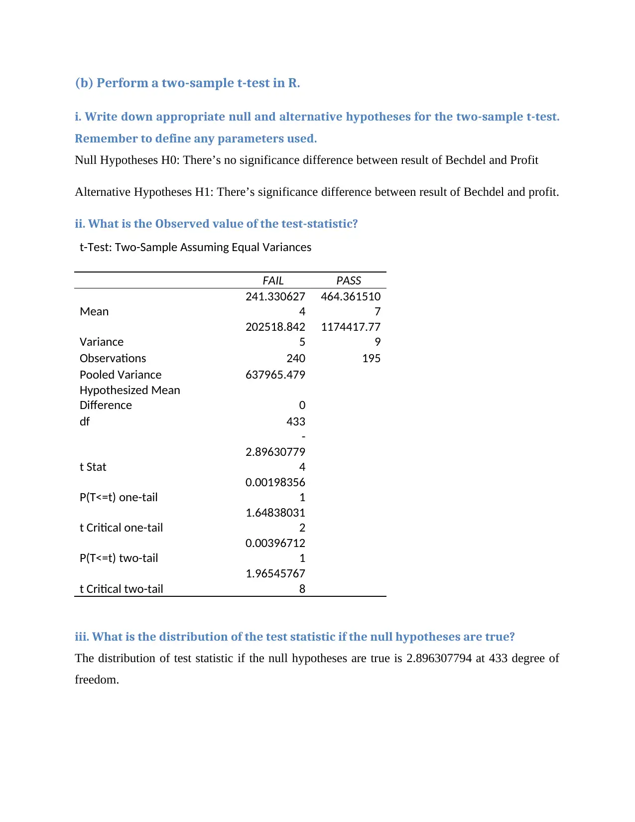
ii. What is the Observed value of the test-statistic?
t-Test: Two-Sample Assuming Equal Variances
FAIL PASS
Mean
241.330627
4
464.361510
7
Variance
202518.842
5
1174417.77
9
Observations 240 195
Pooled Variance 637965.479
Hypothesized Mean
Difference 0
df 433
t Stat
-
2.89630779
4
P(T<=t) one-tail
0.00198356
1
t Critical one-tail
1.64838031
2
P(T<=t) two-tail
0.00396712
1
t Critical two-tail
1.96545767
8
iii. What is the distribution of the test statistic if the null hypotheses are true?
The distribution of test statistic if the null hypotheses are true is 2.896307794 at 433 degree of
freedom.

iv. What is the P-value?
The p value calculated here is two types; upper and lower, as two tailed sample test has been
conducted. The lower tailed p value is 0.002983561 and upper value is 0.003967121.
v. Do you reject or retain the null hypothesis at the 5% significance level? Why?
The two tailed P value is less than level of significance of 0.05 (0.003967121 < P < 0.05); hence
null hypothesis will be rejected and it indicates that there’s significance difference between result
of Bechdel and profit.
(c) Use R to calculate the 95% confidence interval for the difference in the
population mean profit for movies that pass the Bechdel test to those that fail
the Bechdel test. Interpret this confidence interval in context.
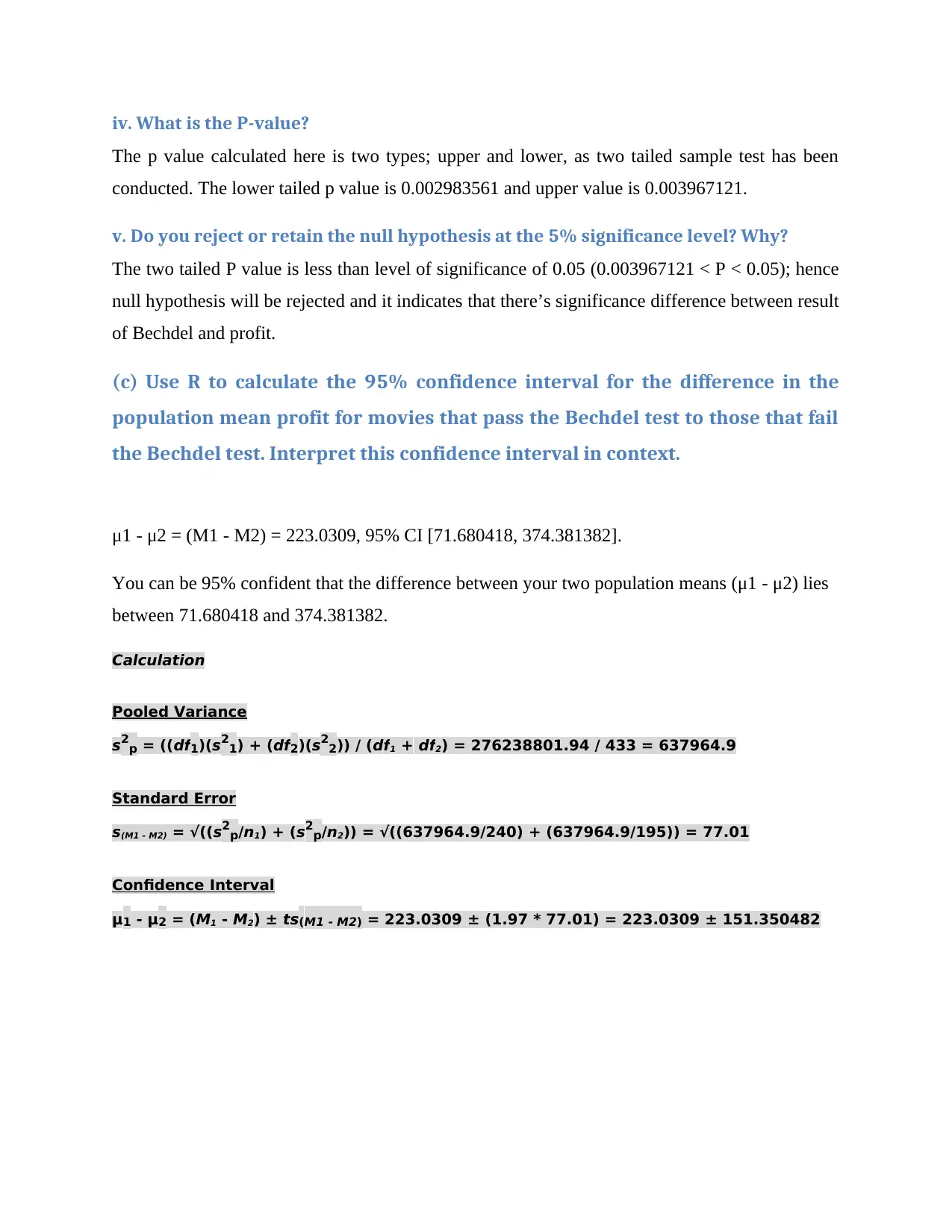
μ1 - μ2 = (M1 - M2) = 223.0309, 95% CI [71.680418, 374.381382].
You can be 95% confident that the difference between your two population means (μ1 - μ2) lies
between 71.680418 and 374.381382.
Calculation
Pooled Variance
s2p = ((df1)(s21) + (df2)(s22)) / (df1 + df2) = 276238801.94 / 433 = 637964.9
Standard Error
s(M1 - M2) = √((s2p/n1) + (s2p/n2)) = √((637964.9/240) + (637964.9/195)) = 77.01
Confidence Interval
μ1 - μ2 = (M1 - M2) ± ts(M1 - M2) = 223.0309 ± (1.97 * 77.01) = 223.0309 ± 151.350482

(d) Produce in R, and include in your submission, appropriate plots to test the
assumption that the observations in each group are from a normal
distribution. Is this assumption reasonable for this dataset? If not, why is the
two-sample t-test still reasonable in this case?
The following assumptions are made by the factual tests depicted in this area. One reason for the
notoriety of the t-test, especially the Aspin-Welch Unequal-Variance t-test, is its strength even
with supposition infringement. Be that as it may, if a supposition that isn't met even around, the
criticalness levels and the intensity of the t-test are refuted. Shockingly, by and by it some of the
time happens that at least one supposition that isn't met. Subsequently, find a way to check the
suspicions before you settle on significant choices dependent on these tests. There are reports in
this method that license you to inspect the suppositions, both outwardly and through suspicions
tests.