Statistical Reasoning in Psychology: ANOVA, Factorial ANOVA, Regression and Chi-Square Tests

This article covers ANOVA, Factorial ANOVA, Regression and Chi-Square Tests in Statistical Reasoning in Psychology. It includes step-by-step analysis of data sets, decision making, and effect size calculation. The article is useful for students of PS390.

ASSIGNMENT 08
PS390 Statistical Reasoning in Psychology
Student Name:
Instructor Name:
Course Number:
12th August 2018

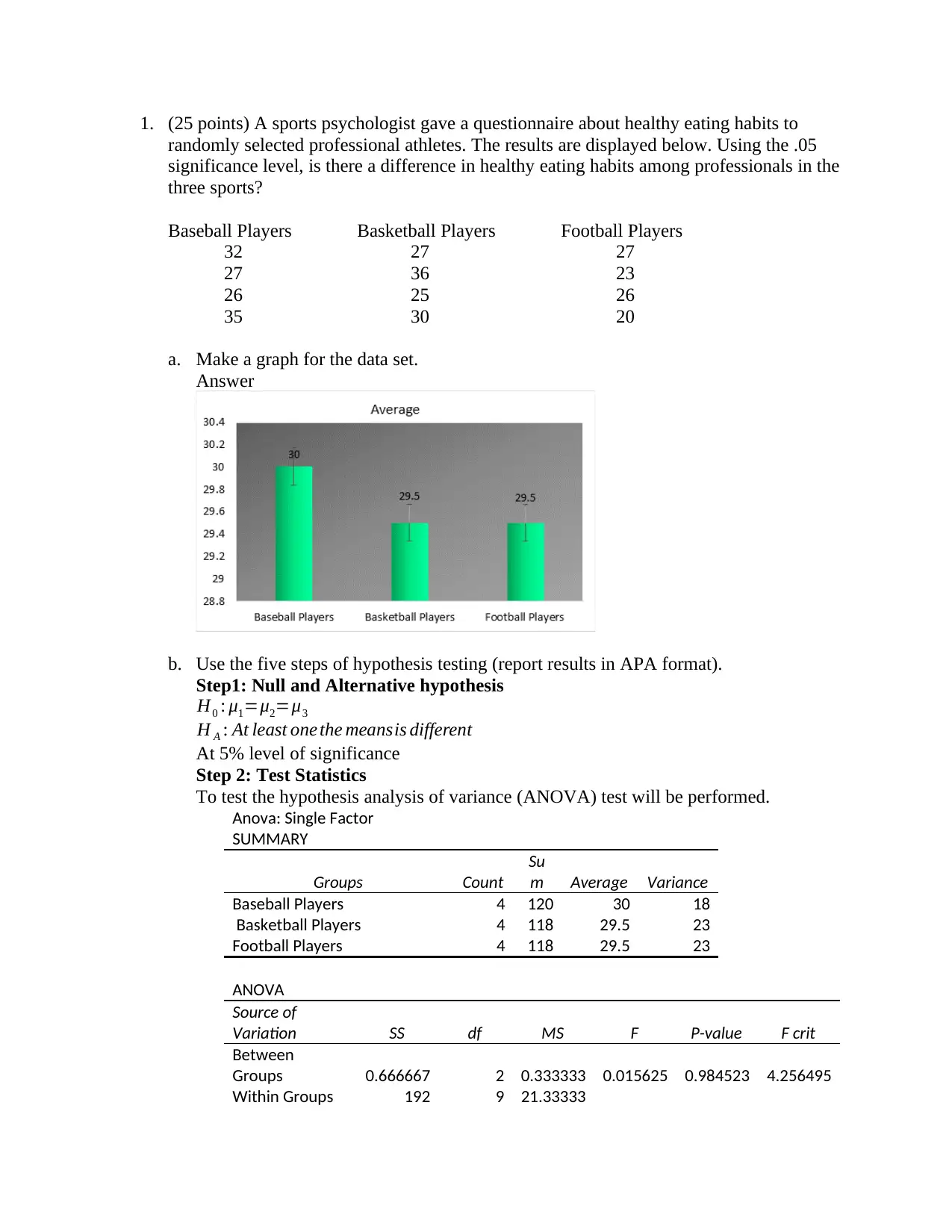
1. (25 points) A sports psychologist gave a questionnaire about healthy eating habits to
randomly selected professional athletes. The results are displayed below. Using the .05
significance level, is there a difference in healthy eating habits among professionals in the
three sports?
Baseball Players Basketball Players Football Players
32 27 27
27 36 23
26 25 26
35 30 20
a. Make a graph for the data set.
Answer
b. Use the five steps of hypothesis testing (report results in APA format).
Step1: Null and Alternative hypothesis
H0 : μ1=μ2=μ3
H A : At least one the meansis different
At 5% level of significance
Step 2: Test Statistics
To test the hypothesis analysis of variance (ANOVA) test will be performed.
Anova: Single Factor
SUMMARY
Groups Count
Su
m Average Variance
Baseball Players 4 120 30 18
Basketball Players 4 118 29.5 23
Football Players 4 118 29.5 23
ANOVA
Source of
Variation SS df MS F P-value F crit
Between
Groups 0.666667 2 0.333333 0.015625 0.984523 4.256495
Within Groups 192 9 21.33333

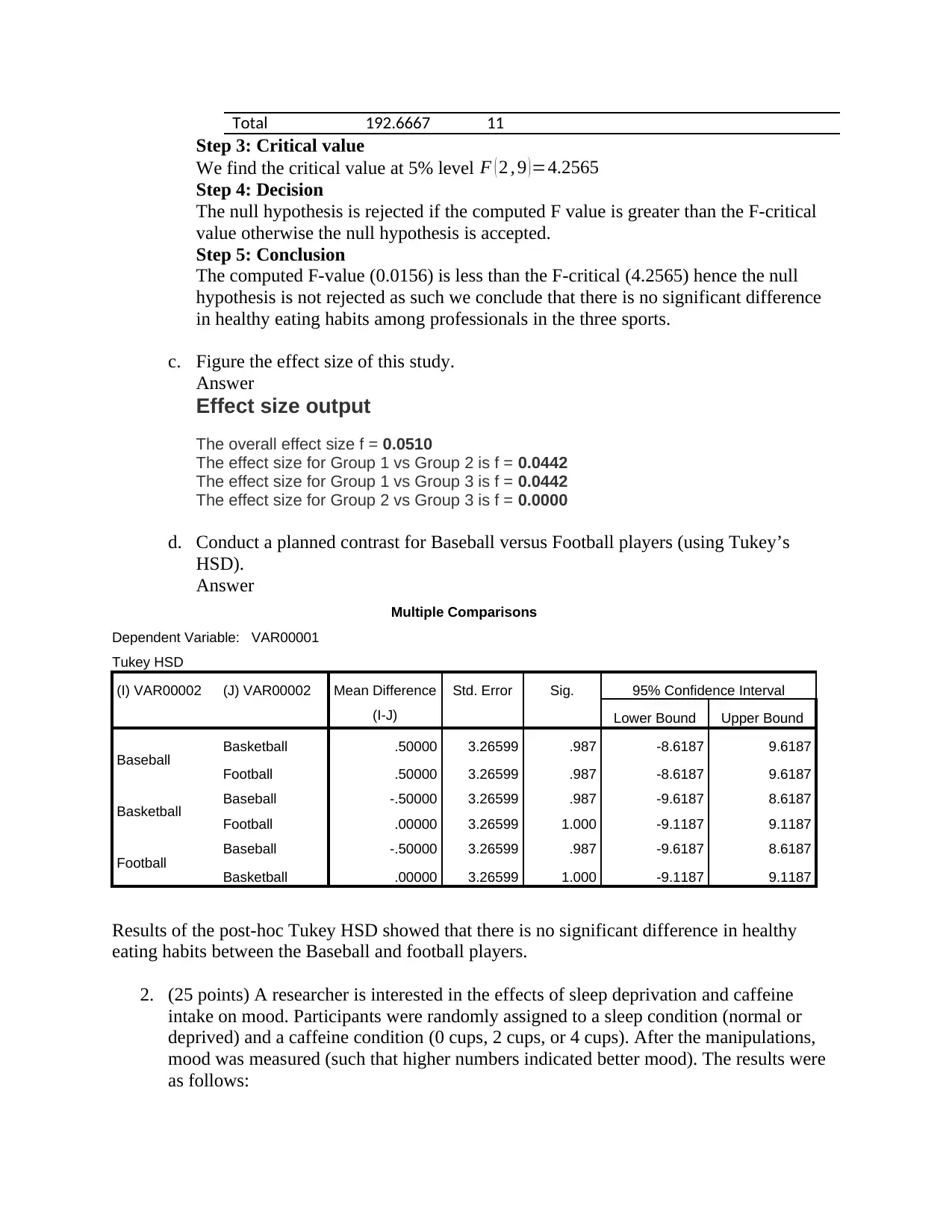
Total 192.6667 11
Step 3: Critical value
We find the critical value at 5% level F ( 2 , 9 )=4.2565
Step 4: Decision
The null hypothesis is rejected if the computed F value is greater than the F-critical
value otherwise the null hypothesis is accepted.
Step 5: Conclusion
The computed F-value (0.0156) is less than the F-critical (4.2565) hence the null
hypothesis is not rejected as such we conclude that there is no significant difference
in healthy eating habits among professionals in the three sports.
c. Figure the effect size of this study.
Answer
Effect size output
The overall effect size f = 0.0510
The effect size for Group 1 vs Group 2 is f = 0.0442
The effect size for Group 1 vs Group 3 is f = 0.0442
The effect size for Group 2 vs Group 3 is f = 0.0000
d. Conduct a planned contrast for Baseball versus Football players (using Tukey’s
HSD).
Answer
Multiple Comparisons
Dependent Variable: VAR00001
Tukey HSD
(I) VAR00002 (J) VAR00002 Mean Difference
(I-J)
Std. Error Sig. 95% Confidence Interval
Lower Bound Upper Bound
Baseball Basketball .50000 3.26599 .987 -8.6187 9.6187
Football .50000 3.26599 .987 -8.6187 9.6187
Basketball Baseball -.50000 3.26599 .987 -9.6187 8.6187
Football .00000 3.26599 1.000 -9.1187 9.1187
Football Baseball -.50000 3.26599 .987 -9.6187 8.6187
Basketball .00000 3.26599 1.000 -9.1187 9.1187
Results of the post-hoc Tukey HSD showed that there is no significant difference in healthy
eating habits between the Baseball and football players.
2. (25 points) A researcher is interested in the effects of sleep deprivation and caffeine
intake on mood. Participants were randomly assigned to a sleep condition (normal or
deprived) and a caffeine condition (0 cups, 2 cups, or 4 cups). After the manipulations,
mood was measured (such that higher numbers indicated better mood). The results were
as follows:

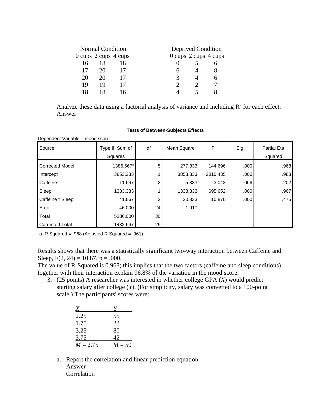
Normal Condition Deprived Condition
0 cups 2 cups 4 cups 0 cups 2 cups 4 cups
16 18 18 0 5 6
17 20 17 6 4 8
20 20 17 3 4 6
19 19 17 2 2 7
18 18 16 4 5 8
Analyze these data using a factorial analysis of variance and including R2 for each effect.
Answer
Tests of Between-Subjects Effects
Dependent Variable: mood score
Source Type III Sum of
Squares
df Mean Square F Sig. Partial Eta
Squared
Corrected Model 1386.667a 5 277.333 144.696 .000 .968
Intercept 3853.333 1 3853.333 2010.435 .000 .988
Caffeine 11.667 2 5.833 3.043 .066 .202
Sleep 1333.333 1 1333.333 695.652 .000 .967
Caffeine * Sleep 41.667 2 20.833 10.870 .000 .475
Error 46.000 24 1.917
Total 5286.000 30
Corrected Total 1432.667 29
a. R Squared = .968 (Adjusted R Squared = .961)
Results shows that there was a statistically significant two-way interaction between Caffeine and
Sleep, F(2, 24) = 10.87, p = .000.
The value of R-Squared is 0.968; this implies that the two factors (caffeine and sleep conditions)
together with their interaction explain 96.8% of the variation in the mood score.
3. (25 points) A researcher was interested in whether college GPA (X) would predict
starting salary after college (Y). (For simplicity, salary was converted to a 100-point
scale.) The participants' scores were:
X Y
2.25 55
1.75 23
3.25 80
3.75 42
M = 2.75 M = 50
a. Report the correlation and linear prediction equation.
Answer
Correlation

X Y
X 1
Y 0.48065 1
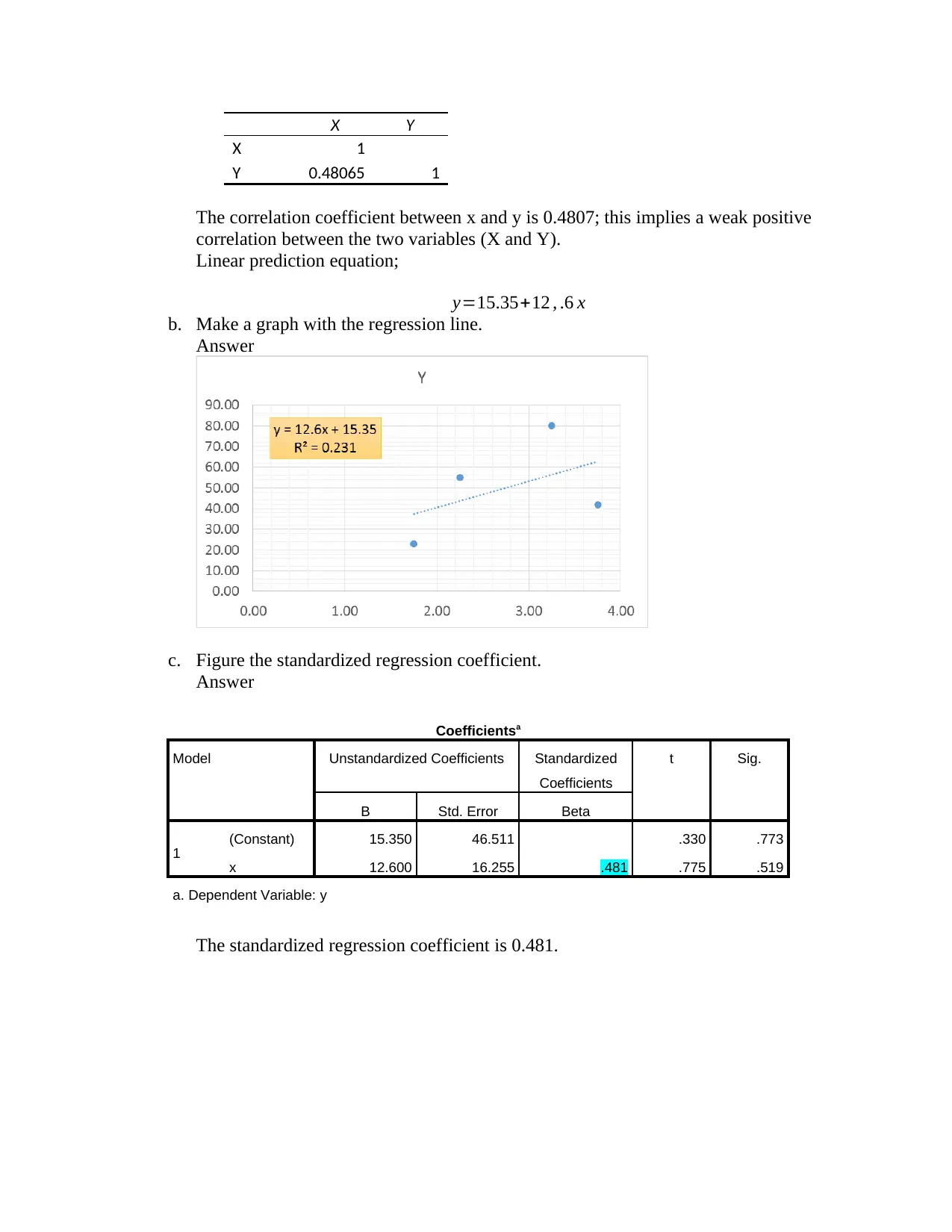
The correlation coefficient between x and y is 0.4807; this implies a weak positive
correlation between the two variables (X and Y).
Linear prediction equation;
y=15.35+12 , .6 x
b. Make a graph with the regression line.
Answer
c. Figure the standardized regression coefficient.
Answer
Coefficientsa
Model Unstandardized Coefficients Standardized
Coefficients
t Sig.
B Std. Error Beta
1 (Constant) 15.350 46.511 .330 .773
x 12.600 16.255 .481 .775 .519
a. Dependent Variable: y
The standardized regression coefficient is 0.481.

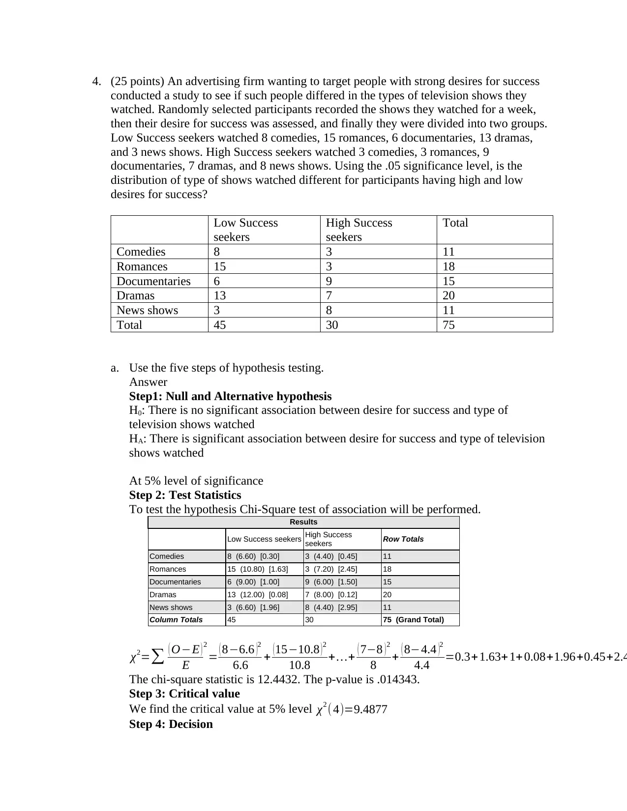
4. (25 points) An advertising firm wanting to target people with strong desires for success
conducted a study to see if such people differed in the types of television shows they
watched. Randomly selected participants recorded the shows they watched for a week,
then their desire for success was assessed, and finally they were divided into two groups.
Low Success seekers watched 8 comedies, 15 romances, 6 documentaries, 13 dramas,
and 3 news shows. High Success seekers watched 3 comedies, 3 romances, 9
documentaries, 7 dramas, and 8 news shows. Using the .05 significance level, is the
distribution of type of shows watched different for participants having high and low
desires for success?
Low Success
seekers
High Success
seekers
Total
Comedies 8 3 11
Romances 15 3 18
Documentaries 6 9 15
Dramas 13 7 20
News shows 3 8 11
Total 45 30 75
a. Use the five steps of hypothesis testing.
Answer
Step1: Null and Alternative hypothesis
H0: There is no significant association between desire for success and type of
television shows watched
HA: There is significant association between desire for success and type of television
shows watched
At 5% level of significance
Step 2: Test Statistics
To test the hypothesis Chi-Square test of association will be performed.
Results
Low Success seekers High Success
seekers Row Totals
Comedies 8 (6.60) [0.30] 3 (4.40) [0.45] 11
Romances 15 (10.80) [1.63] 3 (7.20) [2.45] 18
Documentaries 6 (9.00) [1.00] 9 (6.00) [1.50] 15
Dramas 13 (12.00) [0.08] 7 (8.00) [0.12] 20
News shows 3 (6.60) [1.96] 8 (4.40) [2.95] 11
Column Totals 45 30 75 (Grand Total)
χ2=∑ ( O−E )
E
2
= ( 8−6.6 )2
6.6 + ( 15−10.8 ) 2
10.8 +…+ ( 7−8 ) 2
8 + ( 8−4.4 )2
4.4 =0.3+1.63+1+ 0.08+1.96+0.45+2.4
The chi-square statistic is 12.4432. The p-value is .014343.
Step 3: Critical value
We find the critical value at 5% level χ2 ( 4)=9.4877
Step 4: Decision

The null hypothesis is rejected if the computed Chi-Square value is greater than the
critical Chi-Square value otherwise the null hypothesis is accepted.
Step 5: Conclusion
The computed Chi-Square value (12.4432) is greater than the critical Chi-Square
value (9.4877) hence the null hypothesis is rejected as such we conclude that there is
significant association between desire for success and type of television shows
watched.
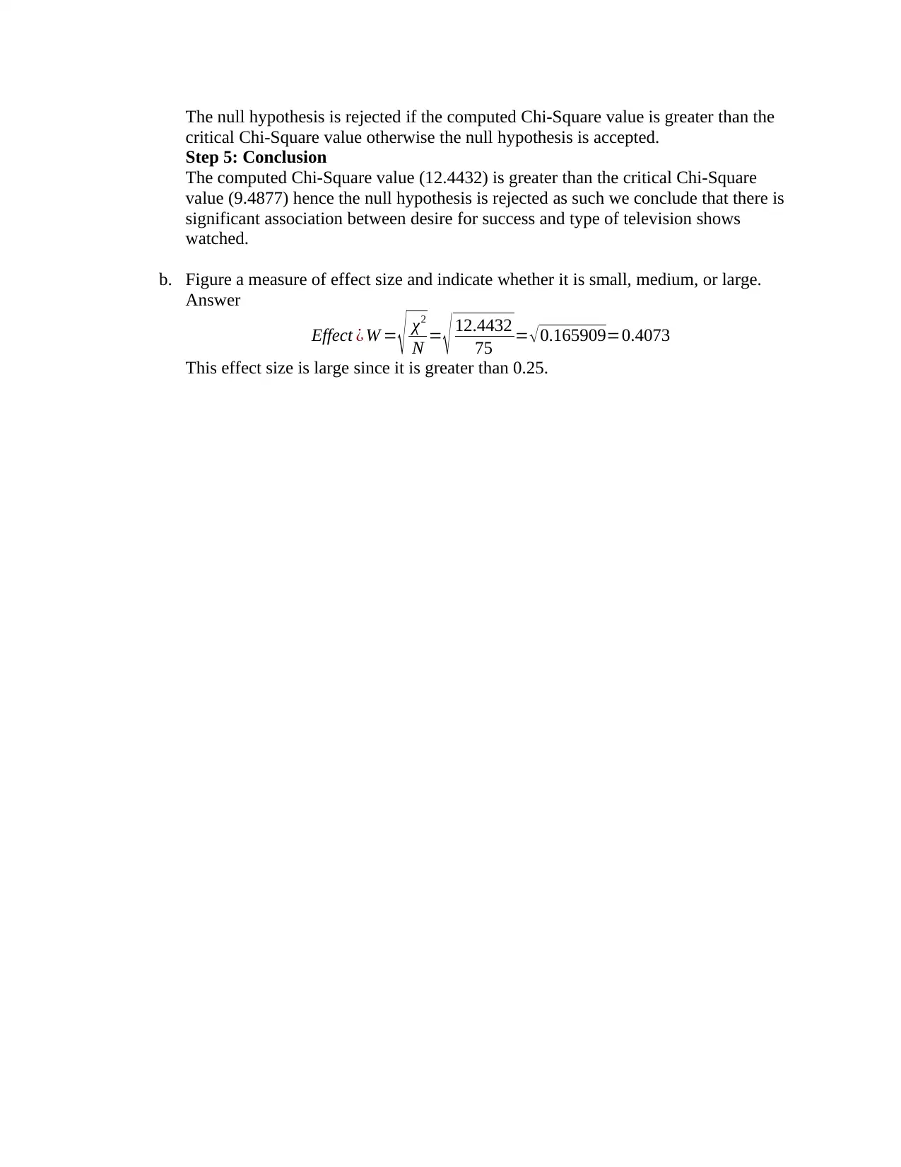
b. Figure a measure of effect size and indicate whether it is small, medium, or large.
Answer
Effect ¿ W = √ χ2
N = √ 12.4432
75 = √0.165909=0.4073
This effect size is large since it is greater than 0.25.