Statistics 2: Dependent t-test, Independent t-test, and ANOVA

This article discusses the application of dependent t-test, independent t-test, and ANOVA in Statistics 2. It includes tables, graphs, and descriptive statistics to support the analysis. The study material is relevant for students taking Statistics 2 course in any college or university.

Running head: STATISTICS 2
Statistics 2
Name of the student
Name of the university
Author’s note

1STATISTICS 2
Table of Contents
Part A: Dependent t-test...................................................................................................................2
Part 1............................................................................................................................................2
Part 2............................................................................................................................................3
Part B: Independent t-test................................................................................................................4
Part 1............................................................................................................................................4
Part 2............................................................................................................................................4
Part 3............................................................................................................................................5
Part 4............................................................................................................................................6
Part C: ANOVA...............................................................................................................................6
Part 1............................................................................................................................................6
Part 2............................................................................................................................................9

2STATISTICS 2
Part A: Dependent t-test
Part 1
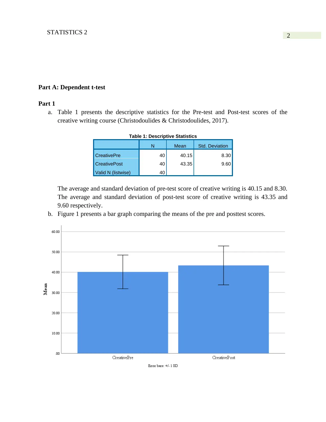
a. Table 1 presents the descriptive statistics for the Pre-test and Post-test scores of the
creative writing course (Christodoulides & Christodoulides, 2017).
Table 1: Descriptive Statistics
N Mean Std. Deviation
CreativePre 40 40.15 8.30
CreativePost 40 43.35 9.60
Valid N (listwise) 40
The average and standard deviation of pre-test score of creative writing is 40.15 and 8.30.
The average and standard deviation of post-test score of creative writing is 43.35 and
9.60 respectively.
b. Figure 1 presents a bar graph comparing the means of the pre and posttest scores.

3STATISTICS 2
Figure 1: Comparison of pre and post test scores.
The comparative distribution of Creativity in Pre-test and Creativity in Post-test indicates that
overall values are greater for Creativity in post-test scores. The score is higher for maximum and
minimum values for post-test score.
c. The Null and Alternate Hypothesis of paired two samples t-test may be written as:
Null Hypothesis (H0): Participation in the creative writing course does not produce any
difference in the mean pre and post-test scores.
H0 : μCreativePre=μCreativePost
Alternate Hypothesis (HA): Participation in the creative writing course does produce
difference in the mean pre and post-test scores (Anderson et al., 2014).
H0 : μCreativePre ≠ μCreativePost
Part 2
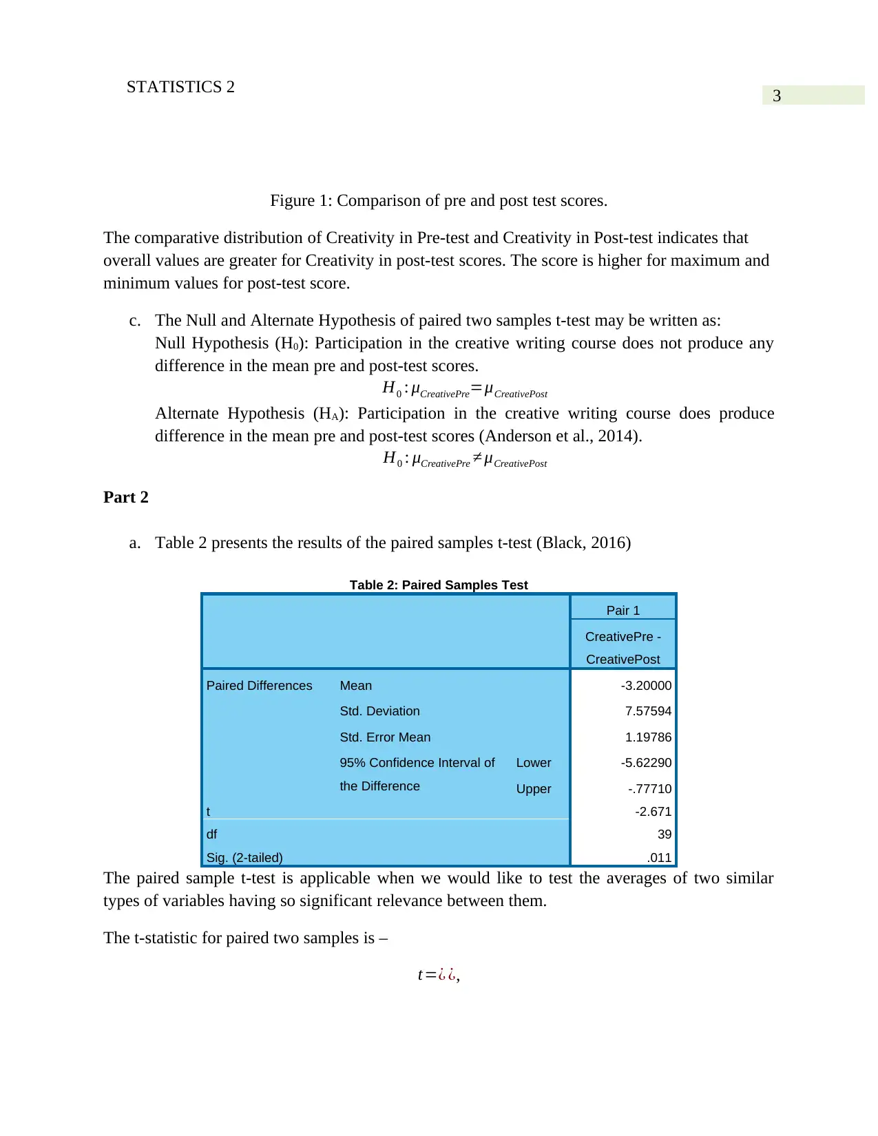
a. Table 2 presents the results of the paired samples t-test (Black, 2016)
Table 2: Paired Samples Test
Pair 1
CreativePre -
CreativePost
Paired Differences Mean -3.20000
Std. Deviation 7.57594
Std. Error Mean 1.19786
95% Confidence Interval of
the Difference
Lower -5.62290
Upper -.77710
t -2.671
df 39
Sig. (2-tailed) .011
The paired sample t-test is applicable when we would like to test the averages of two similar
types of variables having so significant relevance between them.
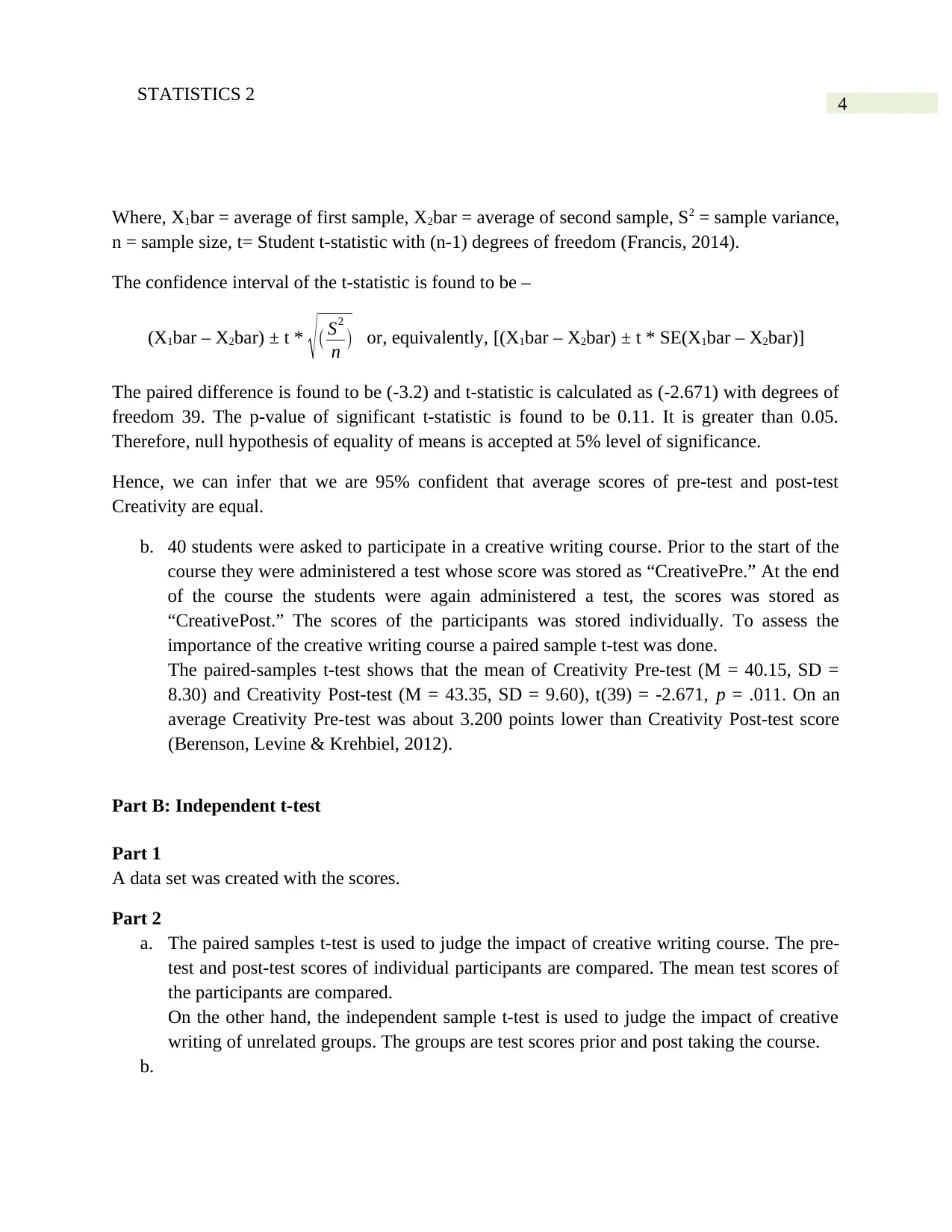
The t-statistic for paired two samples is –
t=¿ ¿,

4STATISTICS 2
Where, X1bar = average of first sample, X2bar = average of second sample, S2 = sample variance,
n = sample size, t= Student t-statistic with (n-1) degrees of freedom (Francis, 2014).
The confidence interval of the t-statistic is found to be –
(X1bar – X2bar) ± t * √( S2
n ) or, equivalently, [(X1bar – X2bar) ± t * SE(X1bar – X2bar)]
The paired difference is found to be (-3.2) and t-statistic is calculated as (-2.671) with degrees of
freedom 39. The p-value of significant t-statistic is found to be 0.11. It is greater than 0.05.
Therefore, null hypothesis of equality of means is accepted at 5% level of significance.
Hence, we can infer that we are 95% confident that average scores of pre-test and post-test
Creativity are equal.
b. 40 students were asked to participate in a creative writing course. Prior to the start of the
course they were administered a test whose score was stored as “CreativePre.” At the end
of the course the students were again administered a test, the scores was stored as
“CreativePost.” The scores of the participants was stored individually. To assess the
importance of the creative writing course a paired sample t-test was done.
The paired-samples t-test shows that the mean of Creativity Pre-test (M = 40.15, SD =
8.30) and Creativity Post-test (M = 43.35, SD = 9.60), t(39) = -2.671, p = .011. On an
average Creativity Pre-test was about 3.200 points lower than Creativity Post-test score
(Berenson, Levine & Krehbiel, 2012).
Part B: Independent t-test
Part 1
A data set was created with the scores.
Part 2
a. The paired samples t-test is used to judge the impact of creative writing course. The pre-
test and post-test scores of individual participants are compared. The mean test scores of
the participants are compared.
On the other hand, the independent sample t-test is used to judge the impact of creative
writing of unrelated groups. The groups are test scores prior and post taking the course.
b.

5STATISTICS 2
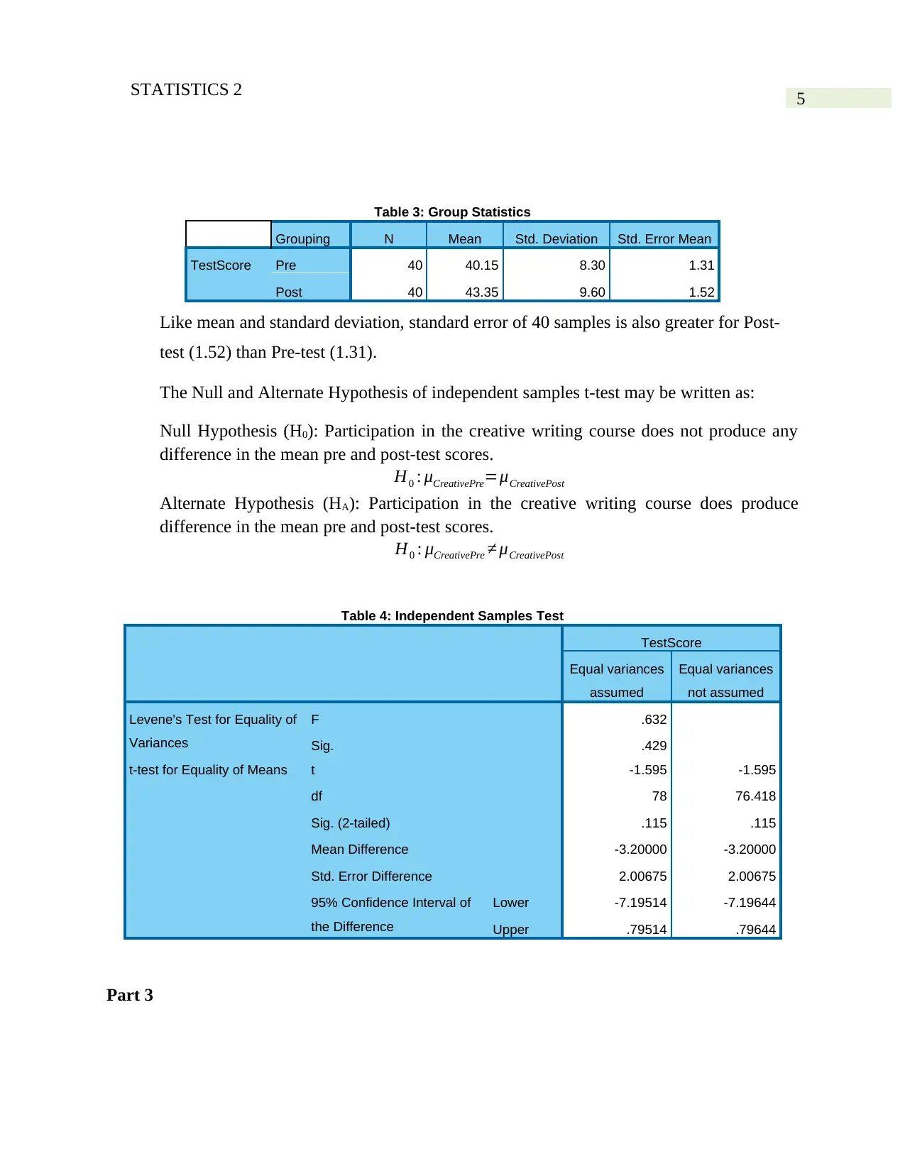
Table 3: Group Statistics
Grouping N Mean Std. Deviation Std. Error Mean
TestScore Pre 40 40.15 8.30 1.31
Post 40 43.35 9.60 1.52
Like mean and standard deviation, standard error of 40 samples is also greater for Post-
test (1.52) than Pre-test (1.31).
The Null and Alternate Hypothesis of independent samples t-test may be written as:
Null Hypothesis (H0): Participation in the creative writing course does not produce any
difference in the mean pre and post-test scores.
H0 : μCreativePre=μCreativePost
Alternate Hypothesis (HA): Participation in the creative writing course does produce
difference in the mean pre and post-test scores.
H0 : μCreativePre ≠ μCreativePost
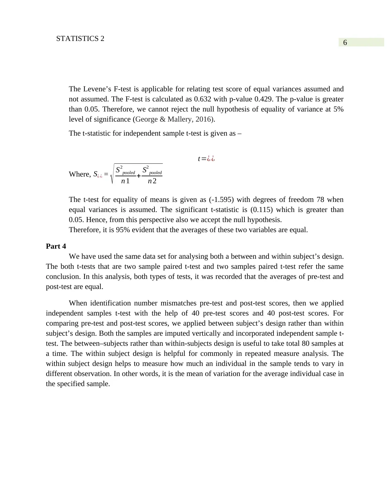
Table 4: Independent Samples Test
TestScore
Equal variances
assumed
Equal variances
not assumed
Levene's Test for Equality of
Variances
F .632
Sig. .429
t-test for Equality of Means t -1.595 -1.595
df 78 76.418
Sig. (2-tailed) .115 .115
Mean Difference -3.20000 -3.20000
Std. Error Difference 2.00675 2.00675
95% Confidence Interval of
the Difference
Lower -7.19514 -7.19644
Upper .79514 .79644
Part 3

6STATISTICS 2
The Levene’s F-test is applicable for relating test score of equal variances assumed and
not assumed. The F-test is calculated as 0.632 with p-value 0.429. The p-value is greater
than 0.05. Therefore, we cannot reject the null hypothesis of equality of variance at 5%
level of significance (George & Mallery, 2016).
The t-statistic for independent sample t-test is given as –
t=¿ ¿
Where, S¿ ¿ = √ S2
pooled
n 1 + S2
pooled
n 2
The t-test for equality of means is given as (-1.595) with degrees of freedom 78 when
equal variances is assumed. The significant t-statistic is (0.115) which is greater than
0.05. Hence, from this perspective also we accept the null hypothesis.
Therefore, it is 95% evident that the averages of these two variables are equal.
Part 4
We have used the same data set for analysing both a between and within subject’s design.
The both t-tests that are two sample paired t-test and two samples paired t-test refer the same
conclusion. In this analysis, both types of tests, it was recorded that the averages of pre-test and
post-test are equal.
When identification number mismatches pre-test and post-test scores, then we applied
independent samples t-test with the help of 40 pre-test scores and 40 post-test scores. For
comparing pre-test and post-test scores, we applied between subject’s design rather than within
subject’s design. Both the samples are imputed vertically and incorporated independent sample t-
test. The between–subjects rather than within-subjects design is useful to take total 80 samples at
a time. The within subject design is helpful for commonly in repeated measure analysis. The
within subject design helps to measure how much an individual in the sample tends to vary in
different observation. In other words, it is the mean of variation for the average individual case in
the specified sample.

7STATISTICS 2
Part C: ANOVA
Part 1
a. The Analysis of variance technique helps to find the differences of mean scores between
Systolic blood pressure and Diastolic blood pressure in Home, Doctor’s Office and
Classroom setting.
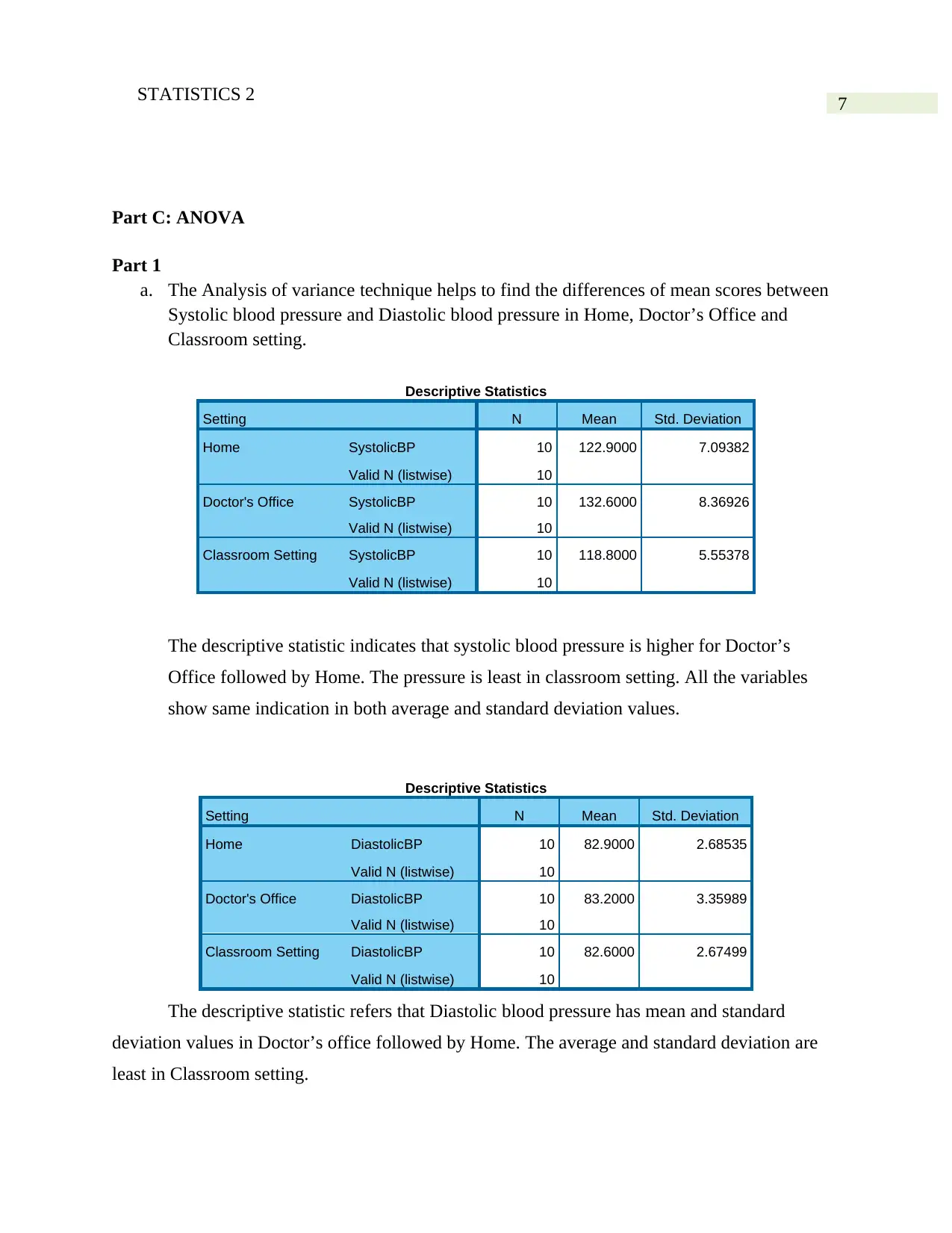
Descriptive Statistics
Setting N Mean Std. Deviation
Home SystolicBP 10 122.9000 7.09382
Valid N (listwise) 10
Doctor's Office SystolicBP 10 132.6000 8.36926
Valid N (listwise) 10
Classroom Setting SystolicBP 10 118.8000 5.55378
Valid N (listwise) 10
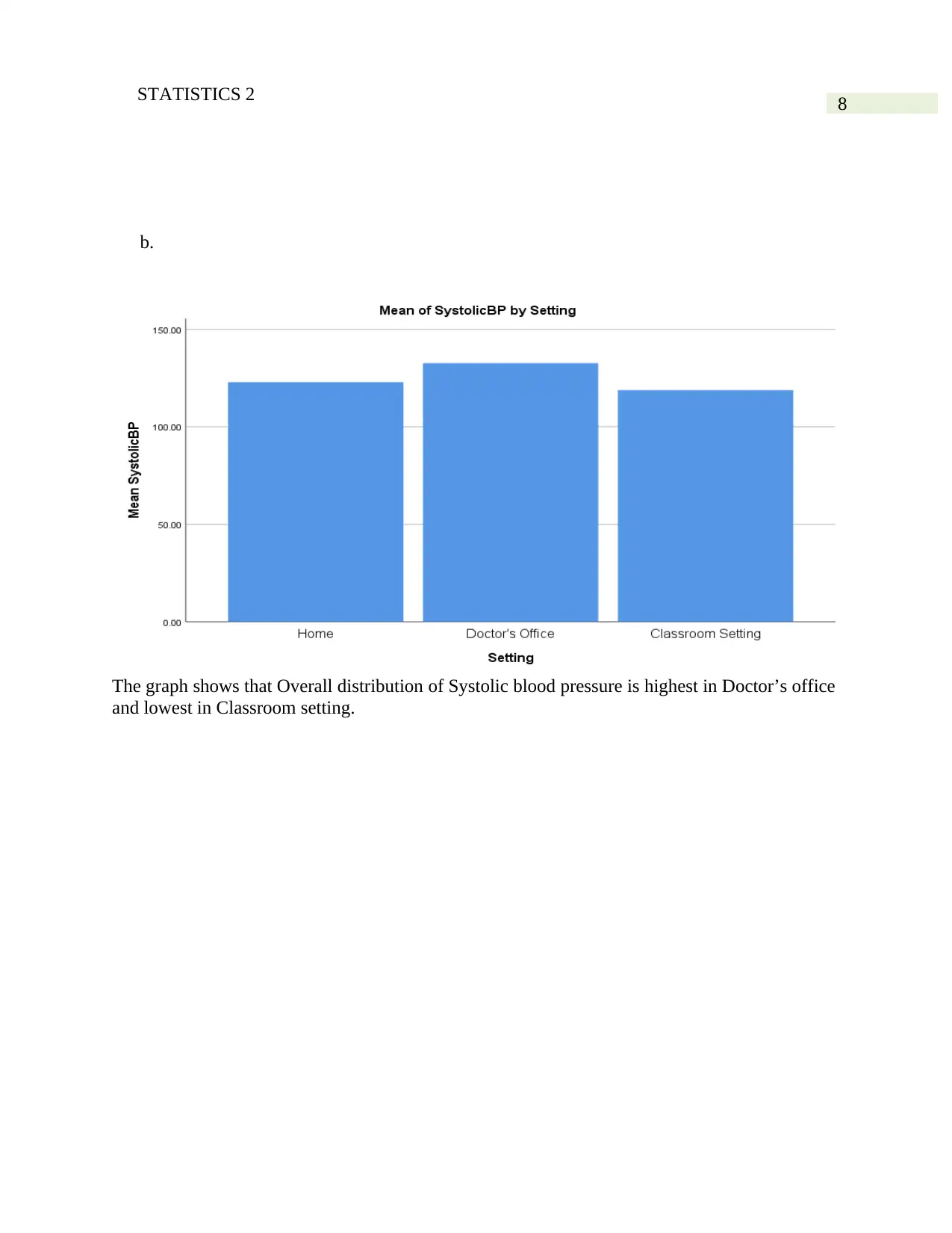
The descriptive statistic indicates that systolic blood pressure is higher for Doctor’s
Office followed by Home. The pressure is least in classroom setting. All the variables
show same indication in both average and standard deviation values.
Descriptive Statistics
Setting N Mean Std. Deviation
Home DiastolicBP 10 82.9000 2.68535
Valid N (listwise) 10
Doctor's Office DiastolicBP 10 83.2000 3.35989
Valid N (listwise) 10
Classroom Setting DiastolicBP 10 82.6000 2.67499
Valid N (listwise) 10
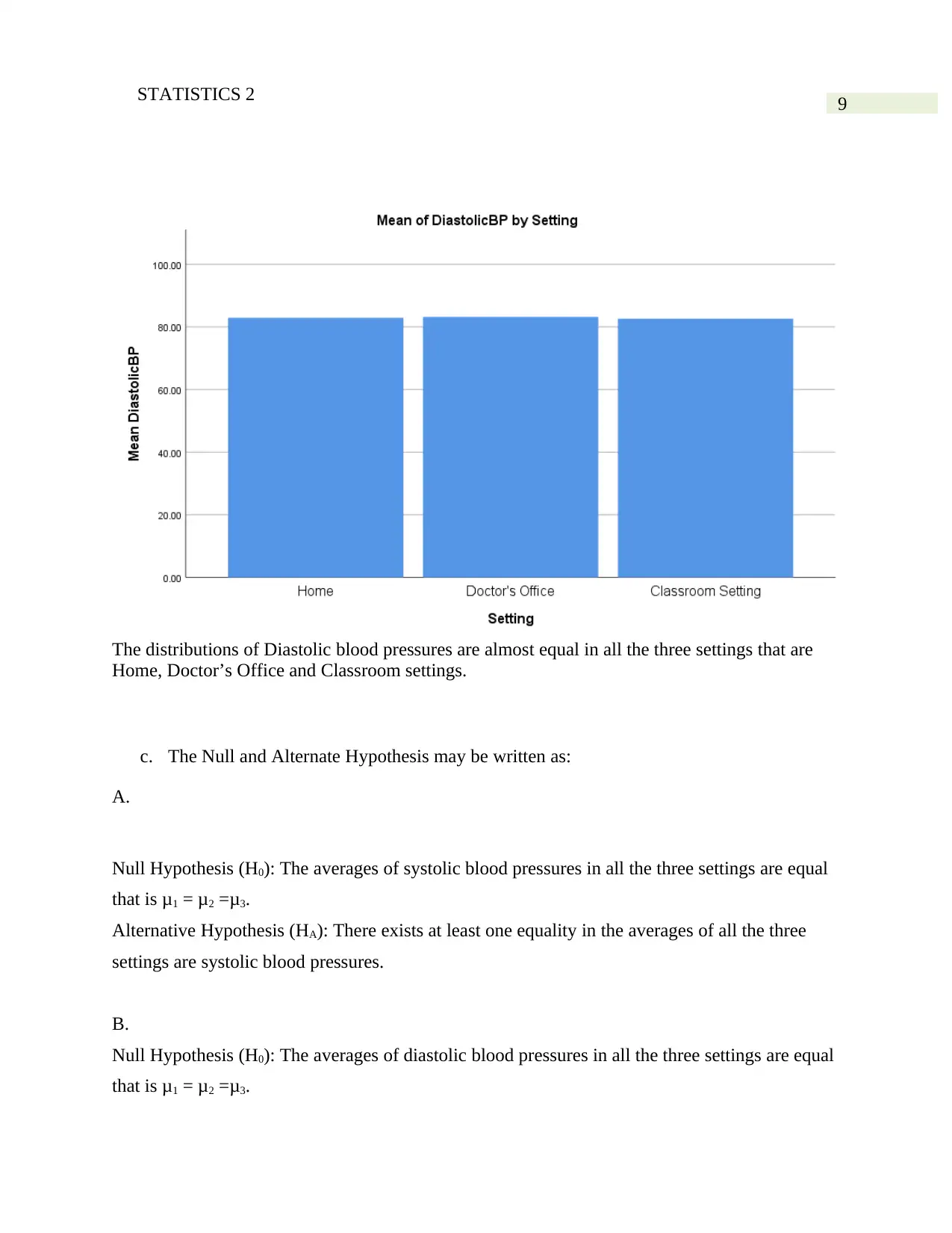
The descriptive statistic refers that Diastolic blood pressure has mean and standard
deviation values in Doctor’s office followed by Home. The average and standard deviation are
least in Classroom setting.

8STATISTICS 2
b.
The graph shows that Overall distribution of Systolic blood pressure is highest in Doctor’s office
and lowest in Classroom setting.

9STATISTICS 2
The distributions of Diastolic blood pressures are almost equal in all the three settings that are
Home, Doctor’s Office and Classroom settings.
c. The Null and Alternate Hypothesis may be written as:
A.
Null Hypothesis (H0): The averages of systolic blood pressures in all the three settings are equal
that is μ1 = μ2 =μ3.
Alternative Hypothesis (HA): There exists at least one equality in the averages of all the three
settings are systolic blood pressures.
B.
Null Hypothesis (H0): The averages of diastolic blood pressures in all the three settings are equal
that is μ1 = μ2 =μ3.

10STATISTICS 2
Alternative Hypothesis (HA): There exists at least one equality in the averages of all the three
settings are diastolic blood pressures.
Part 2
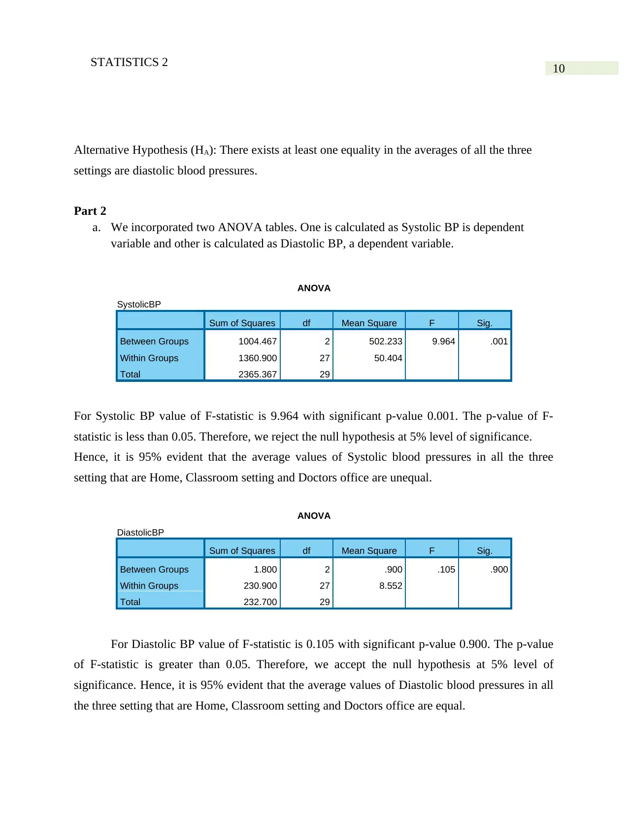
a. We incorporated two ANOVA tables. One is calculated as Systolic BP is dependent
variable and other is calculated as Diastolic BP, a dependent variable.
ANOVA
SystolicBP
Sum of Squares df Mean Square F Sig.
Between Groups 1004.467 2 502.233 9.964 .001
Within Groups 1360.900 27 50.404
Total 2365.367 29
For Systolic BP value of F-statistic is 9.964 with significant p-value 0.001. The p-value of F-
statistic is less than 0.05. Therefore, we reject the null hypothesis at 5% level of significance.
Hence, it is 95% evident that the average values of Systolic blood pressures in all the three
setting that are Home, Classroom setting and Doctors office are unequal.
ANOVA
DiastolicBP
Sum of Squares df Mean Square F Sig.
Between Groups 1.800 2 .900 .105 .900
Within Groups 230.900 27 8.552
Total 232.700 29
For Diastolic BP value of F-statistic is 0.105 with significant p-value 0.900. The p-value
of F-statistic is greater than 0.05. Therefore, we accept the null hypothesis at 5% level of
significance. Hence, it is 95% evident that the average values of Diastolic blood pressures in all
the three setting that are Home, Classroom setting and Doctors office are equal.

11STATISTICS 2
b. The Sum of squares within groups and between groups are significantly higher in case of
ANOVA test of Systolic BP. On the other hand, sum of squares between groups is
insignificant than within group SSE in the ANOVA table of Diastolic blood pressure
(Field, 2013).
Multiple Comparisons
Dependent Variable: SystolicBP
Bonferroni
(I) Setting (J) Setting
Mean Difference
(I-J) Std. Error Sig.
95% Confidence Interval
Lower Bound Upper Bound
Home Doctor's Office -9.70000* 3.17502 .015 -17.8041 -1.5959
Classroom Setting 4.10000 3.17502 .623 -4.0041 12.2041
Doctor's Office Home 9.70000* 3.17502 .015 1.5959 17.8041
Classroom Setting 13.80000* 3.17502 .001 5.6959 21.9041
Classroom Setting Home -4.10000 3.17502 .623 -12.2041 4.0041
Doctor's Office -13.80000* 3.17502 .001 -21.9041 -5.6959
*. The mean difference is significant at the 0.05 level.
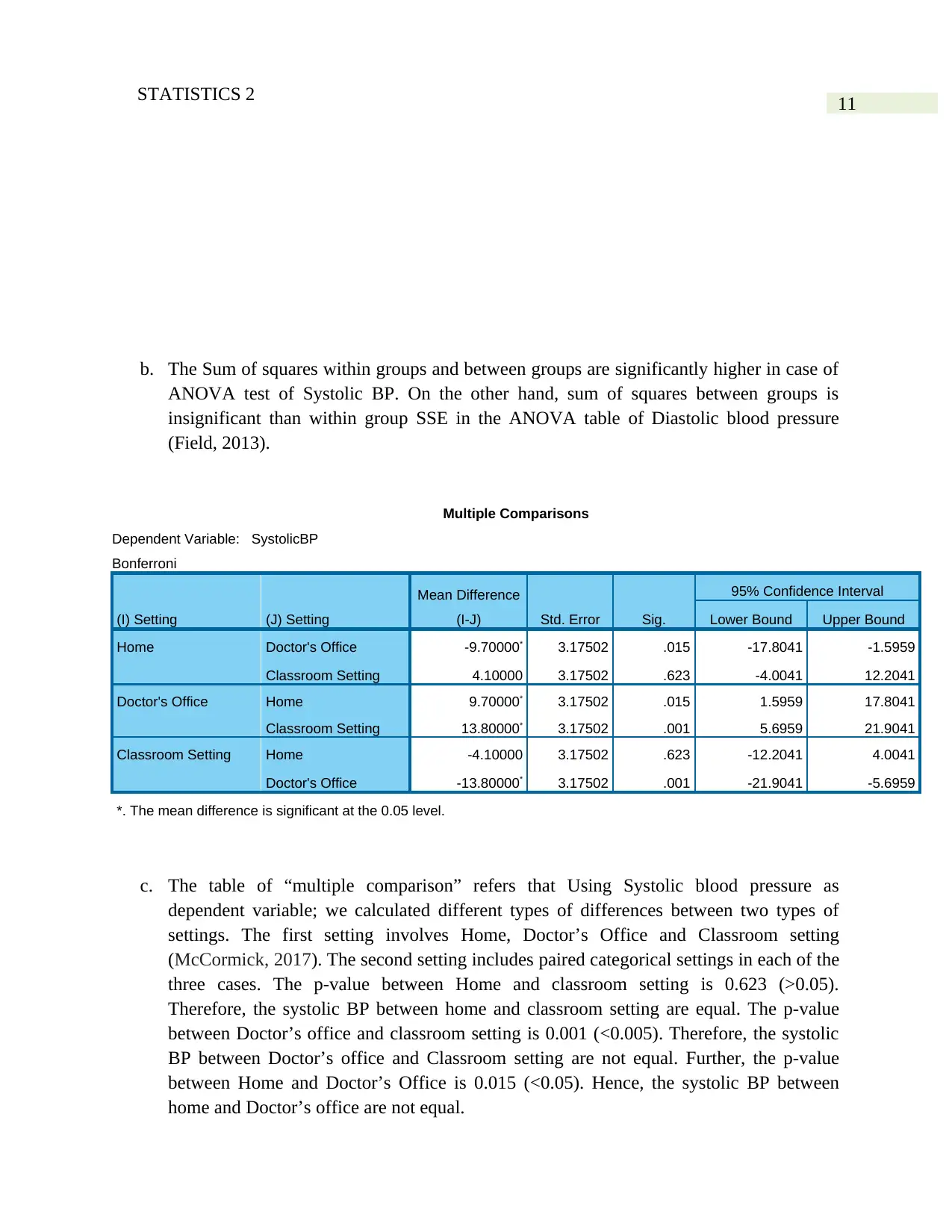
c. The table of “multiple comparison” refers that Using Systolic blood pressure as
dependent variable; we calculated different types of differences between two types of
settings. The first setting involves Home, Doctor’s Office and Classroom setting
(McCormick, 2017). The second setting includes paired categorical settings in each of the
three cases. The p-value between Home and classroom setting is 0.623 (>0.05).
Therefore, the systolic BP between home and classroom setting are equal. The p-value
between Doctor’s office and classroom setting is 0.001 (<0.005). Therefore, the systolic
BP between Doctor’s office and Classroom setting are not equal. Further, the p-value
between Home and Doctor’s Office is 0.015 (<0.05). Hence, the systolic BP between
home and Doctor’s office are not equal.

12STATISTICS 2

13STATISTICS 2
References
Anderson, D. R., Sweeney, D. J., Williams, T. A., Camm, J. D., & Cochran, J. J.
(2014). Essentials of statistics for business and economics. Cengage Learning.
Berenson, M. L., Levine, D. M., & Krehbiel, T. C. (2012). Basic business statistics. Upper
Saddle River, NJ: Prentice Hall.
Black, K. (2016). Business statistics: Contemporary decision making. John Wiley & Sons.
Christodoulides, C., & Christodoulides, G. (2017). Analysis and Presentation of Experimental
Results. Springer
Field, A. (2013). Discovering statistics using IBM SPSS statistics. Sage.
Francis, A. (2014). Business mathematics and statistics. Cengage Learning EMEA.
George, D., & Mallery, P. (2016). IBM SPSS Statistics 23 step by step: A simple guide and
reference. Routledge.
McCormick, K., Salcedo, J., Peck, J., & Wheeler, A. (2017). SPSS Statistics for data analysis
and visualization. John Wiley & Sons.