Statistics: Frequency Analysis, Linear Regression, ANOVA and Multiple Regression

This article covers frequency analysis and graphical representation of examination scores, linear regression model, one-way ANOVA table, and multiple regression model. It also includes tables and figures for better understanding.

Running Head: STATISTICS
Statistics
Name of the student:
Name of the university:
Course ID:

1STATISTICS
Table of Contents
Answer 1..........................................................................................................................................2
Answer 2..........................................................................................................................................3
Answer 3..........................................................................................................................................4
Answer 4..........................................................................................................................................5
References:......................................................................................................................................9
Table of tables
Table 1: The table of frequency distribution, cumulative frequency distribution, relative
frequency distribution, cumulative frequency distribution and percent frequency distribution of
examination scores of 20 students...................................................................................................2
Table 2: Linear Regression Model_1..............................................................................................3
Table 3: One-way ANOVA table....................................................................................................4
Table 4: Multiple Regression Model...............................................................................................6
Table 5: Linear Regression Model_2..............................................................................................7
Table of Figures
Figure 1: Histogram of frequency in percentages as per examination scores.................................2
Figure 2: Bar chart of average scores of four countries...................................................................5

2STATISTICS
Answer 1.
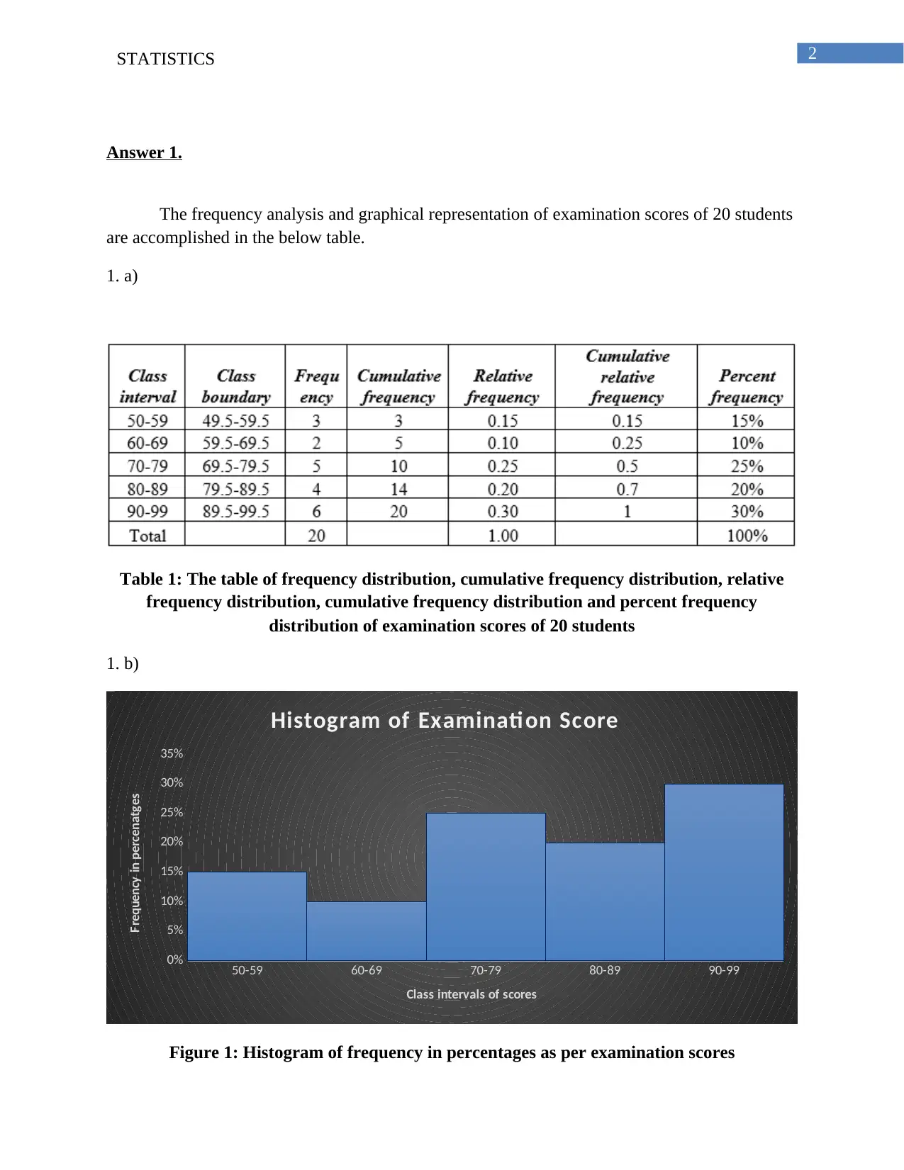
The frequency analysis and graphical representation of examination scores of 20 students
are accomplished in the below table.
1. a)
Table 1: The table of frequency distribution, cumulative frequency distribution, relative
frequency distribution, cumulative frequency distribution and percent frequency
distribution of examination scores of 20 students
1. b)
50-59 60-69 70-79 80-89 90-99
0%
5%
10%
15%
20%
25%
30%
35%
Histogram of Examination Score
Class intervals of scores
Frequency in percenatges
Figure 1: Histogram of frequency in percentages as per examination scores

3STATISTICS
The shape of the distribution of Examination score indicates that the examination score is
left-skewed. Its right tail is longer than its left tail. Its mode is greater than median and the
median is greater than mean.
Answer 2.
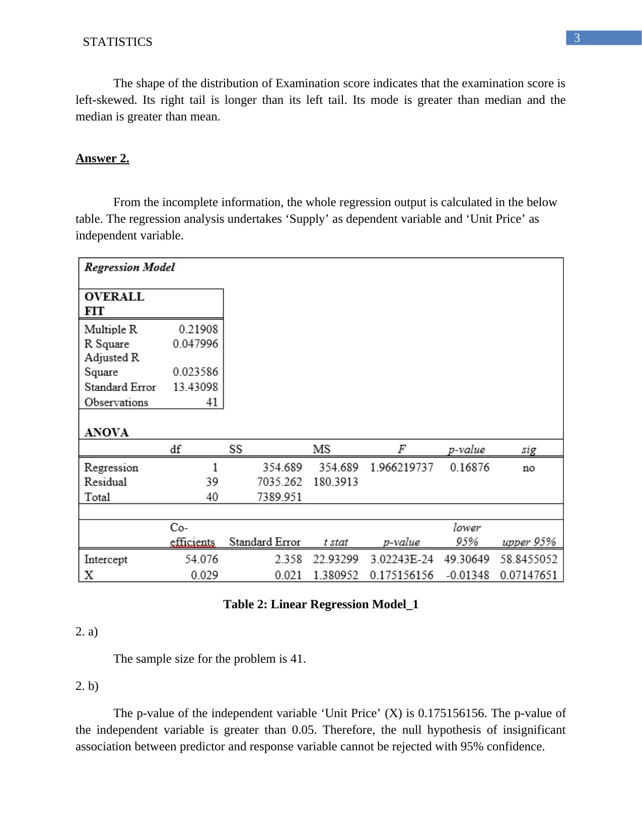
From the incomplete information, the whole regression output is calculated in the below
table. The regression analysis undertakes ‘Supply’ as dependent variable and ‘Unit Price’ as
independent variable.
Table 2: Linear Regression Model_1
2. a)
The sample size for the problem is 41.
2. b)
The p-value of the independent variable ‘Unit Price’ (X) is 0.175156156. The p-value of
the independent variable is greater than 0.05. Therefore, the null hypothesis of insignificant
association between predictor and response variable cannot be rejected with 95% confidence.

4STATISTICS
It could be interpreted that ‘Unit Price (X)’ and ‘Supply’ (Y) are not statistically and
linearly associated to each other (Yao and Li 2014).
2. c)
The calculated ‘Co-efficient of determination’ is 0.047996.
The ‘Co-efficient of determination’ (R2) denotes the power of independent variable that
explains the variability of dependent variable (Moorad and Wade 2013). The value of co-
efficient of determination refers that ‘Unit Price (X)’ explains 4.80% variation of the dependent
variable ‘Supply (Y)’.
2. d)
The co-efficient of correlation (R = 0.21908) indicates that supply is very weakly
correlated to the unit price (Wang et al. 2013). The dependent variable has almost no link with
the independent variable.
2. e)
The linear regression model is given as, Y = 54.076 + 0.029*X
When the unit price (X) is $50,000, then the supply would be-
Y = 54.076 + 0.029*50000 = 1504.076.
The estimated supply is 1504.076 units.
Answer 3.
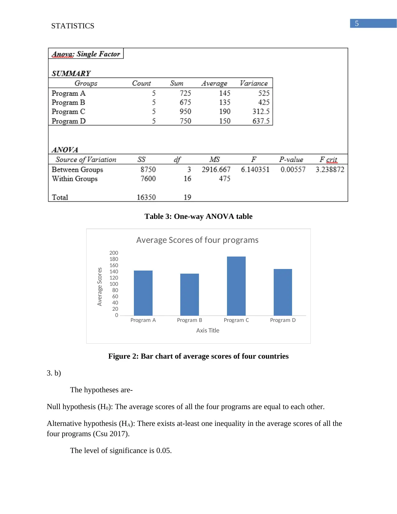
The outputs of 20 randomly selected employees with respect to their program groups (A,
B, C and D) are provided in the assignment table. To test the equality of productivity averages of
four kinds of programs, the one-way ANOVA testing is executed.
3. a)

5STATISTICS
Table 3: One-way ANOVA table
Program A Program B Program C Program D
0
20
40
60
80
100
120
140
160
180
200
Average Scores of four programs
Axis Title
Average Scores
Figure 2: Bar chart of average scores of four countries
3. b)
The hypotheses are-
Null hypothesis (H0): The average scores of all the four programs are equal to each other.
Alternative hypothesis (HA): There exists at-least one inequality in the average scores of all the
four programs (Csu 2017).
The level of significance is 0.05.

6STATISTICS
The calculated p-value of the F-statistic (6.140351) is 0.00557. The p-value is less than
5%. Also, the Fcal (6.140351) is higher than Fcrit (3.238872). Therefore, we can reject the null
hypothesis with 95% confidence (Bates et al. 2014); also, the alternative hypothesis could be
accepted.
The productivity of workers of Program C has higher average than Program A, Program
B and Program D. It could be recommended that the line programmers of Program C are more
effective than any other program and hence more accepted in the context of productivity.
Answer 4.
The data set of a company records the data of weekly sales of products (y) as dependent
variable and unit price of the competitor’s product (x1) as well as advertising expenditures (x2) as
independent variables.

7STATISTICS
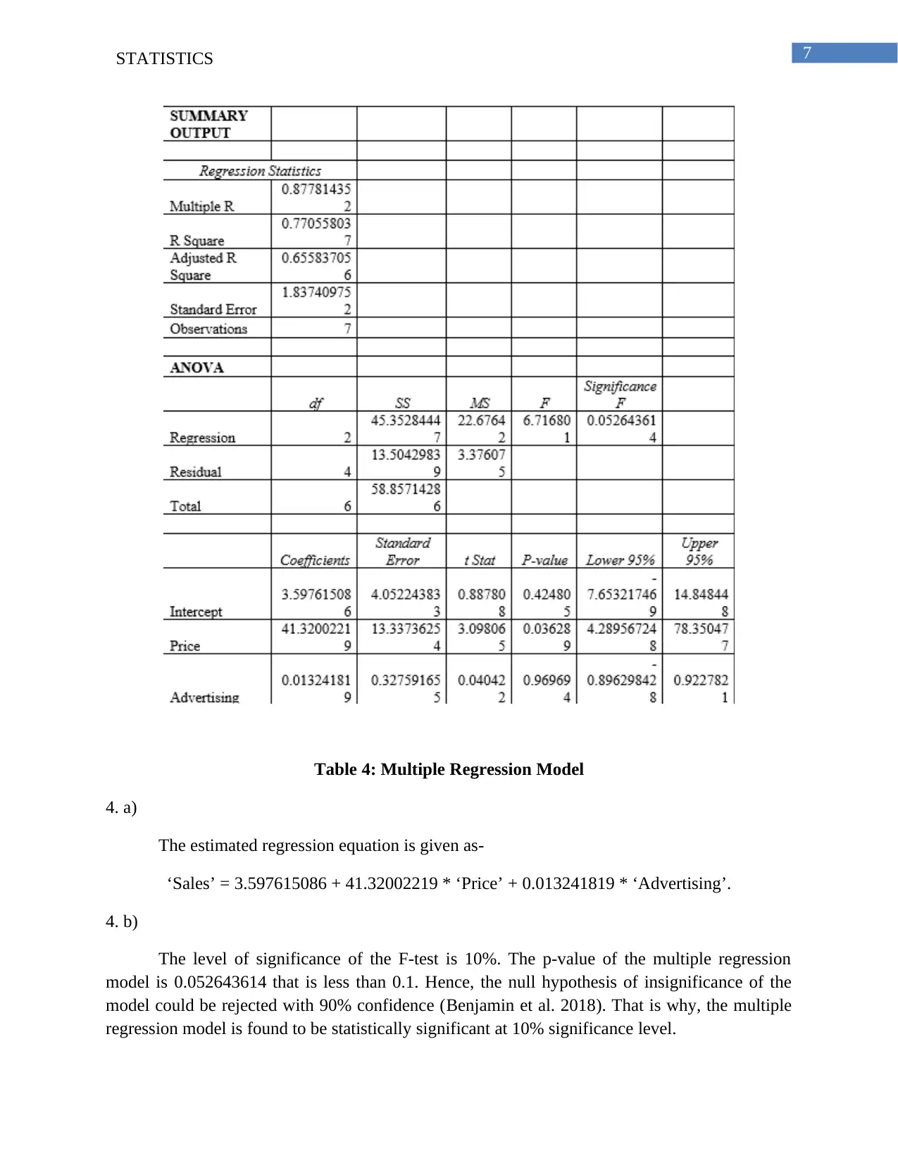
Table 4: Multiple Regression Model
4. a)
The estimated regression equation is given as-
‘Sales’ = 3.597615086 + 41.32002219 * ‘Price’ + 0.013241819 * ‘Advertising’.
4. b)
The level of significance of the F-test is 10%. The p-value of the multiple regression
model is 0.052643614 that is less than 0.1. Hence, the null hypothesis of insignificance of the
model could be rejected with 90% confidence (Benjamin et al. 2018). That is why, the multiple
regression model is found to be statistically significant at 10% significance level.

8STATISTICS
4. c)
The p-values of the independent variables are respectively-
 Price (0.036289).
 Advertising (0.969694).
The p-value of ‘Price’ is less than 5% and p-value of ‘Advertising’ is greater than 5%.
Therefore, out of these two predictor variables, ‘Price’ is the significant factor and ‘Advertising’
is the insignificant factor.
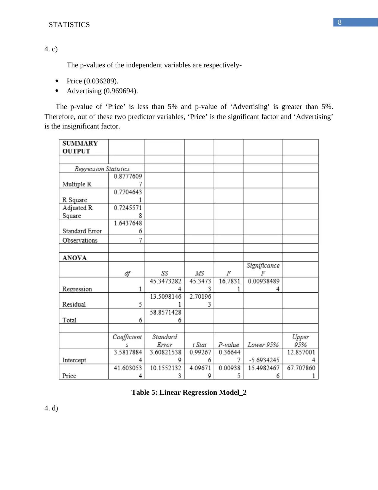
Table 5: Linear Regression Model_2
4. d)

9STATISTICS
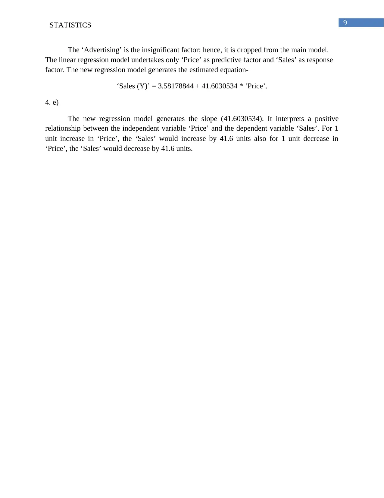
The ‘Advertising’ is the insignificant factor; hence, it is dropped from the main model.
The linear regression model undertakes only ‘Price’ as predictive factor and ‘Sales’ as response
factor. The new regression model generates the estimated equation-
‘Sales (Y)’ = 3.58178844 + 41.6030534 * ‘Price’.
4. e)
The new regression model generates the slope (41.6030534). It interprets a positive
relationship between the independent variable ‘Price’ and the dependent variable ‘Sales’. For 1
unit increase in ‘Price’, the ‘Sales’ would increase by 41.6 units also for 1 unit decrease in
‘Price’, the ‘Sales’ would decrease by 41.6 units.

10STATISTICS
References:
Bates, D., Maechler, M., Bolker, B. and Walker, S., 2014. lme4: Linear mixed-effects models
using Eigen and S4. R package version, 1(7), pp.1-23.
Benjamin, D.J., Berger, J.O., Johannesson, M., Nosek, B.A., Wagenmakers, E.J., Berk, R.,
Bollen, K.A., Brembs, B., Brown, L., Camerer, C. and Cesarini, D., 2018. Redefine statistical
significance. Nature Human Behaviour, 2(1), p.6.
CSU, C.M., 2017. Analysis of variance. Analysis, (1/49).
Moorad, J.A. and Wade, M.J., 2013. Selection gradients, the opportunity for selection, and the
coefficient of determination. The American Naturalist, 181(3), pp.291-300.
Wang, G.J., Xie, C., Chen, S., Yang, J.J. and Yang, M.Y., 2013. Random matrix theory analysis
of cross-correlations in the US stock market: Evidence from Pearson’s correlation coefficient and
detrended cross-correlation coefficient. Physica A: statistical mechanics and its
applications, 392(17), pp.3715-3730.
Yao, W. and Li, L., 2014. A new regression model: modal linear regression. Scandinavian
Journal of Statistics, 41(3), pp.656-671.