Statistics and Data Analysis

This document explores the puzzle of Burgernomics and the factors influencing purchasing power parity using statistics and data analysis. It discusses the findings from the Big Mac Index and HDI data, and analyzes the correlation between HDI index and variables such as life expectancy, schooling, and GNI per capita.

Statistics and Data Analysis 1
Statistics and Data Analysis
Name
Course Number
Date
Faculty Name

Statistics and Data Analysis 2
Statistics and Data Analysis
Burgernomics
a) The puzzle from the theoretical perspective of Burgernomics based on the findings of the
Big Mac Index 2016
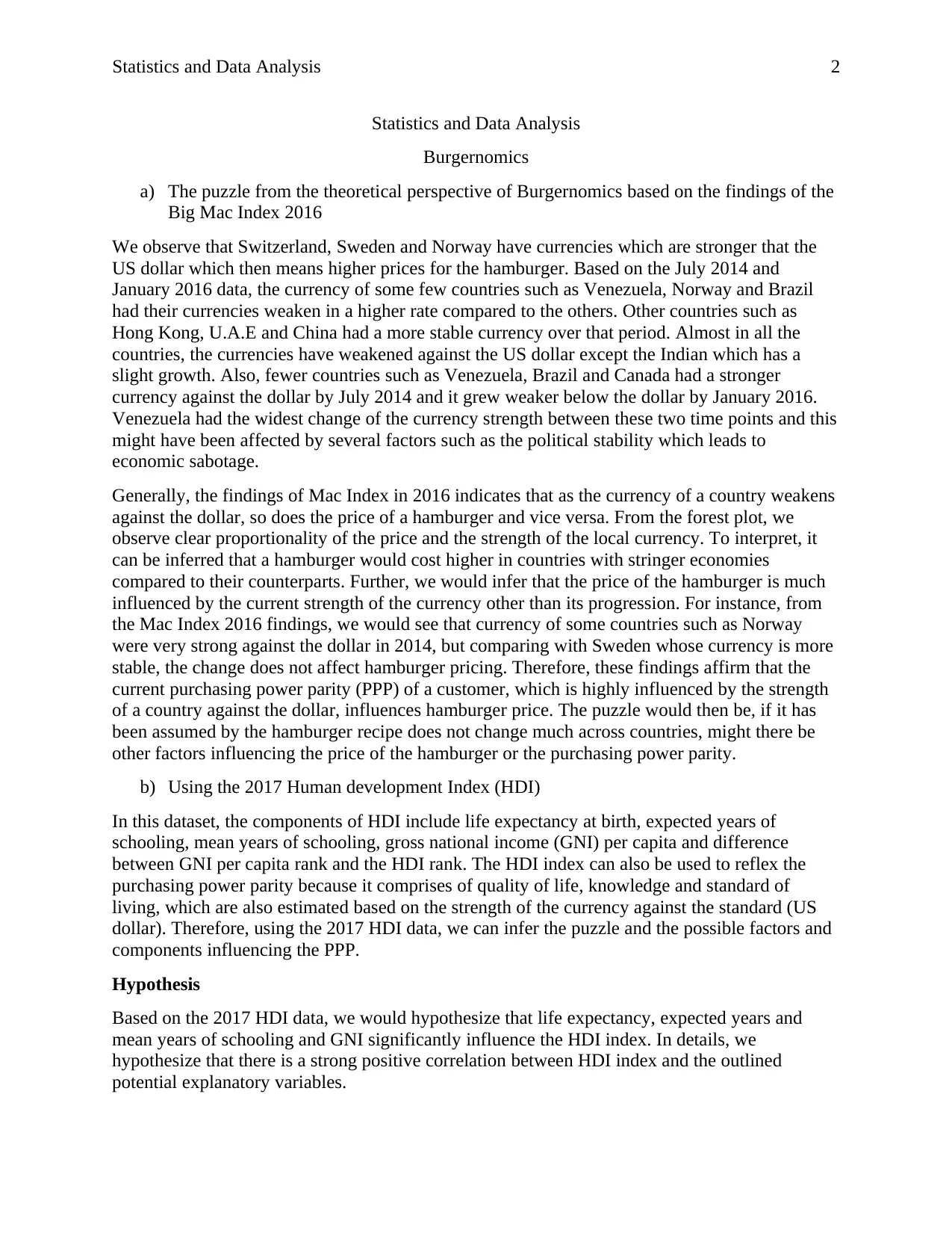
We observe that Switzerland, Sweden and Norway have currencies which are stronger that the
US dollar which then means higher prices for the hamburger. Based on the July 2014 and
January 2016 data, the currency of some few countries such as Venezuela, Norway and Brazil
had their currencies weaken in a higher rate compared to the others. Other countries such as
Hong Kong, U.A.E and China had a more stable currency over that period. Almost in all the
countries, the currencies have weakened against the US dollar except the Indian which has a
slight growth. Also, fewer countries such as Venezuela, Brazil and Canada had a stronger
currency against the dollar by July 2014 and it grew weaker below the dollar by January 2016.
Venezuela had the widest change of the currency strength between these two time points and this
might have been affected by several factors such as the political stability which leads to
economic sabotage.
Generally, the findings of Mac Index in 2016 indicates that as the currency of a country weakens
against the dollar, so does the price of a hamburger and vice versa. From the forest plot, we
observe clear proportionality of the price and the strength of the local currency. To interpret, it
can be inferred that a hamburger would cost higher in countries with stringer economies
compared to their counterparts. Further, we would infer that the price of the hamburger is much
influenced by the current strength of the currency other than its progression. For instance, from
the Mac Index 2016 findings, we would see that currency of some countries such as Norway
were very strong against the dollar in 2014, but comparing with Sweden whose currency is more
stable, the change does not affect hamburger pricing. Therefore, these findings affirm that the
current purchasing power parity (PPP) of a customer, which is highly influenced by the strength
of a country against the dollar, influences hamburger price. The puzzle would then be, if it has
been assumed by the hamburger recipe does not change much across countries, might there be
other factors influencing the price of the hamburger or the purchasing power parity.
b) Using the 2017 Human development Index (HDI)
In this dataset, the components of HDI include life expectancy at birth, expected years of
schooling, mean years of schooling, gross national income (GNI) per capita and difference
between GNI per capita rank and the HDI rank. The HDI index can also be used to reflex the
purchasing power parity because it comprises of quality of life, knowledge and standard of
living, which are also estimated based on the strength of the currency against the standard (US
dollar). Therefore, using the 2017 HDI data, we can infer the puzzle and the possible factors and
components influencing the PPP.
Hypothesis
Based on the 2017 HDI data, we would hypothesize that life expectancy, expected years and
mean years of schooling and GNI significantly influence the HDI index. In details, we
hypothesize that there is a strong positive correlation between HDI index and the outlined
potential explanatory variables.

Statistics and Data Analysis 3
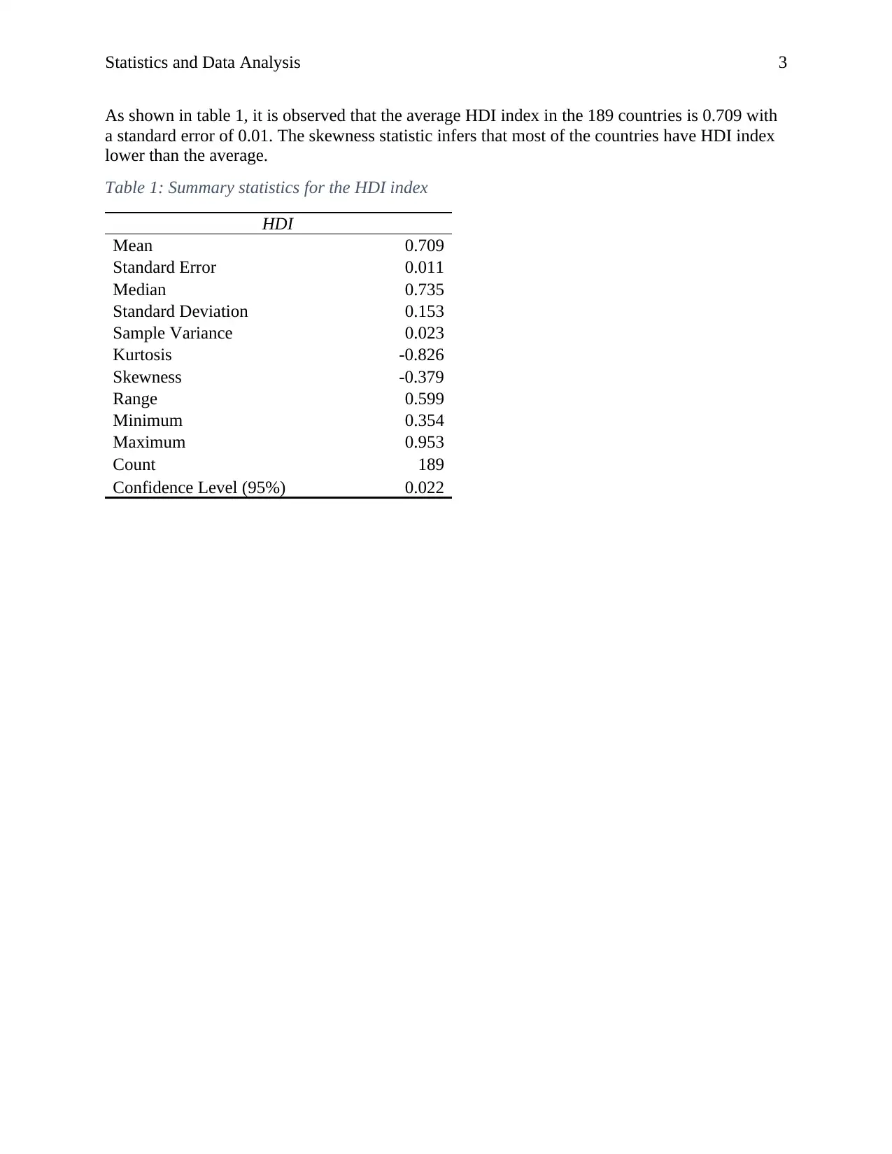
As shown in table 1, it is observed that the average HDI index in the 189 countries is 0.709 with
a standard error of 0.01. The skewness statistic infers that most of the countries have HDI index
lower than the average.
Table 1: Summary statistics for the HDI index
HDI
Mean 0.709
Standard Error 0.011
Median 0.735
Standard Deviation 0.153
Sample Variance 0.023
Kurtosis -0.826
Skewness -0.379
Range 0.599
Minimum 0.354
Maximum 0.953
Count 189
Confidence Level (95%) 0.022

Statistics and Data Analysis 4
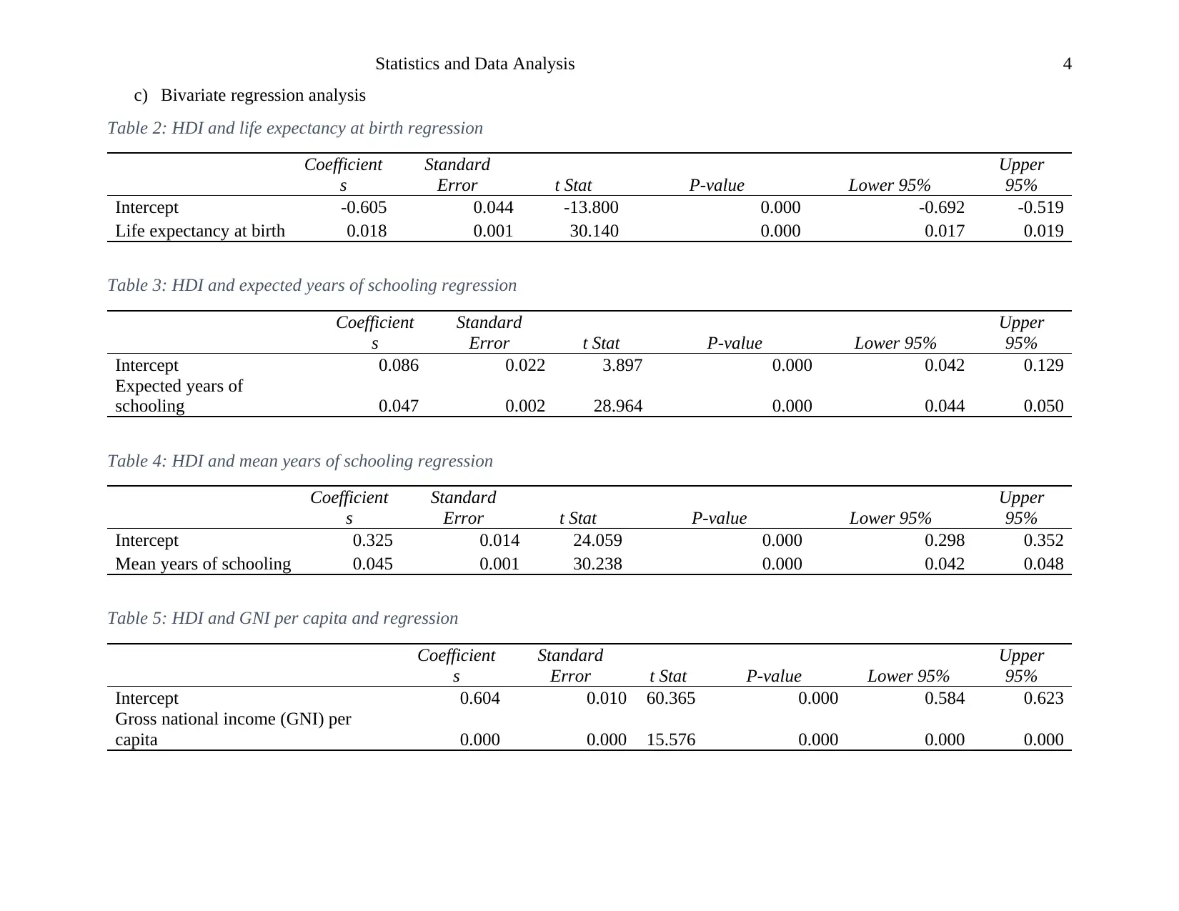
c) Bivariate regression analysis
Table 2: HDI and life expectancy at birth regression
Coefficient
s
Standard
Error t Stat P-value Lower 95%
Upper
95%
Intercept -0.605 0.044 -13.800 0.000 -0.692 -0.519
Life expectancy at birth 0.018 0.001 30.140 0.000 0.017 0.019
Table 3: HDI and expected years of schooling regression
Coefficient
s
Standard
Error t Stat P-value Lower 95%
Upper
95%
Intercept 0.086 0.022 3.897 0.000 0.042 0.129
Expected years of
schooling 0.047 0.002 28.964 0.000 0.044 0.050
Table 4: HDI and mean years of schooling regression
Coefficient
s
Standard
Error t Stat P-value Lower 95%
Upper
95%
Intercept 0.325 0.014 24.059 0.000 0.298 0.352
Mean years of schooling 0.045 0.001 30.238 0.000 0.042 0.048
Table 5: HDI and GNI per capita and regression
Coefficient
s
Standard
Error t Stat P-value Lower 95%
Upper
95%
Intercept 0.604 0.010 60.365 0.000 0.584 0.623
Gross national income (GNI) per
capita 0.000 0.000 15.576 0.000 0.000 0.000

Statistics and Data Analysis 5
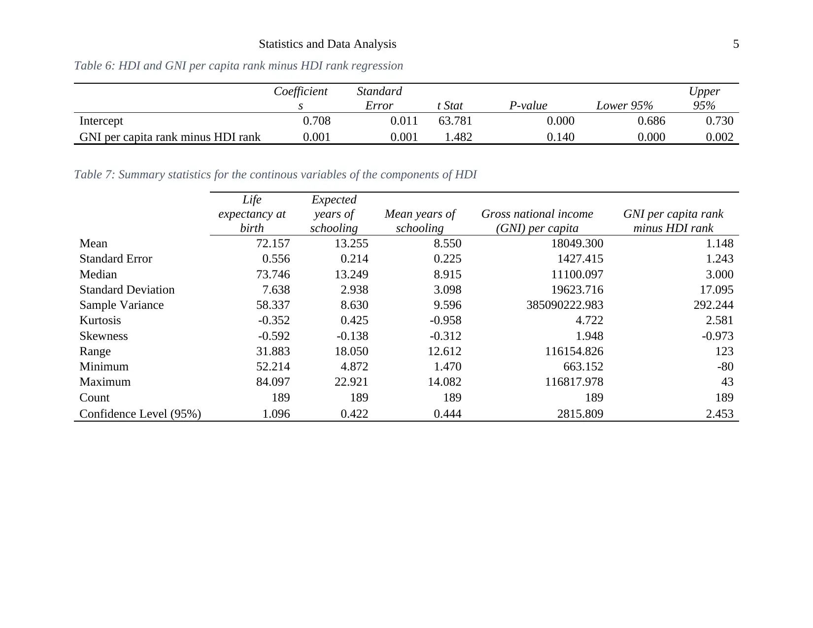
Table 6: HDI and GNI per capita rank minus HDI rank regression
Coefficient
s
Standard
Error t Stat P-value Lower 95%
Upper
95%
Intercept 0.708 0.011 63.781 0.000 0.686 0.730
GNI per capita rank minus HDI rank 0.001 0.001 1.482 0.140 0.000 0.002
Table 7: Summary statistics for the continous variables of the components of HDI
Life
expectancy at
birth
Expected
years of
schooling
Mean years of
schooling
Gross national income
(GNI) per capita
GNI per capita rank
minus HDI rank
Mean 72.157 13.255 8.550 18049.300 1.148
Standard Error 0.556 0.214 0.225 1427.415 1.243
Median 73.746 13.249 8.915 11100.097 3.000
Standard Deviation 7.638 2.938 3.098 19623.716 17.095
Sample Variance 58.337 8.630 9.596 385090222.983 292.244
Kurtosis -0.352 0.425 -0.958 4.722 2.581
Skewness -0.592 -0.138 -0.312 1.948 -0.973
Range 31.883 18.050 12.612 116154.826 123
Minimum 52.214 4.872 1.470 663.152 -80
Maximum 84.097 22.921 14.082 116817.978 43
Count 189 189 189 189 189
Confidence Level (95%) 1.096 0.422 0.444 2815.809 2.453

Statistics and Data Analysis 6
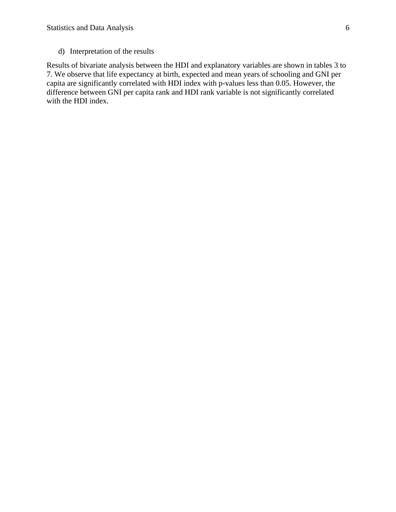
d) Interpretation of the results
Results of bivariate analysis between the HDI and explanatory variables are shown in tables 3 to
7. We observe that life expectancy at birth, expected and mean years of schooling and GNI per
capita are significantly correlated with HDI index with p-values less than 0.05. However, the
difference between GNI per capita rank and HDI rank variable is not significantly correlated
with the HDI index.