Statistics and Research Methods for Business Decision Making

This document provides information on Australian exports, store's umbrella sales, and the relationship between final consumption and retail turnover. It includes graphs, numerical summaries, and regression analysis. The document is relevant for the course Statistics and Research Methods for Business Decision Making.

STATISTICS AND RESEARCH METHODS FOR BUSINESS DECISION MAKING
Student’s Name
Code + Name of Course
Professor’s Name
University
City (State)
Date
1

Question 1: Australian Exports
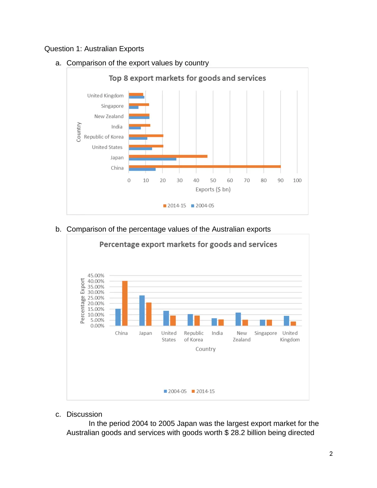
a. Comparison of the export values by country
b. Comparison of the percentage values of the Australian exports
c. Discussion
In the period 2004 to 2005 Japan was the largest export market for the
Australian goods and services with goods worth $ 28.2 billion being directed
2

towards this market. This trend took a huge turn in 2014 -2015 period where
China bypassed Japan to be at the top of the Australian good’s market. From the
graph in (a) above it is evident that the exports from Australia to Japan did go up
between the two period, the growth rate was though slower than for the Chinese
market-oriented goods. India, Singapore, UK and New Zealand remained in the
list of top markets for the Australian goods and services despite the little growth
rate of the quantity of goods and services directed to the markets.
The graph in (b) shows that as at 2015, China was importing over 40% of
all the goods and services that were exported from Australia, this was followed
closely by Japan which was taking around 20.85% of the goods and services.
One of the significant observations from this chart is the drop in the percentage
exports to Japan from 27% to 20% between the year 2005 and 2015. On the
other hand, goods and services destined for China grew from 15% to 40%. Both
US, Korea, India, New Zealand, Singapore as well as UK saw their imports from
Australia drop within the two periods.
Question 2: Store’s Umbrella sales
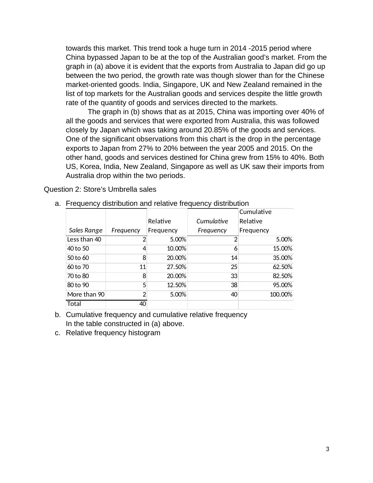
a. Frequency distribution and relative frequency distribution
Sales Range Frequency
Relative
Frequency
Cumulative
Frequency
Cumulative
Relative
Frequency
Less than 40 2 5.00% 2 5.00%
40 to 50 4 10.00% 6 15.00%
50 to 60 8 20.00% 14 35.00%
60 to 70 11 27.50% 25 62.50%
70 to 80 8 20.00% 33 82.50%
80 to 90 5 12.50% 38 95.00%
More than 90 2 5.00% 40 100.00%
Total 40
b. Cumulative frequency and cumulative relative frequency
In the table constructed in (a) above.
c. Relative frequency histogram
3

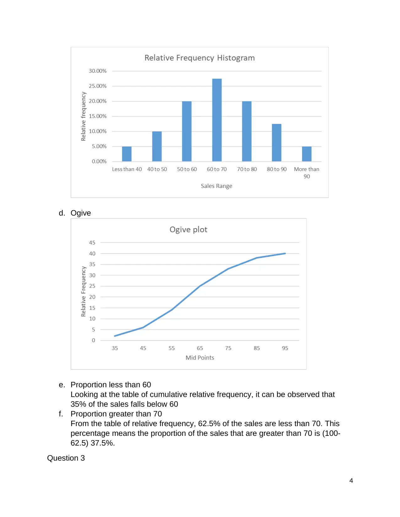
d. Ogive
e. Proportion less than 60
Looking at the table of cumulative relative frequency, it can be observed that
35% of the sales falls below 60
f. Proportion greater than 70
From the table of relative frequency, 62.5% of the sales are less than 70. This
percentage means the proportion of the sales that are greater than 70 is (100-
62.5) 37.5%.
Question 3
4

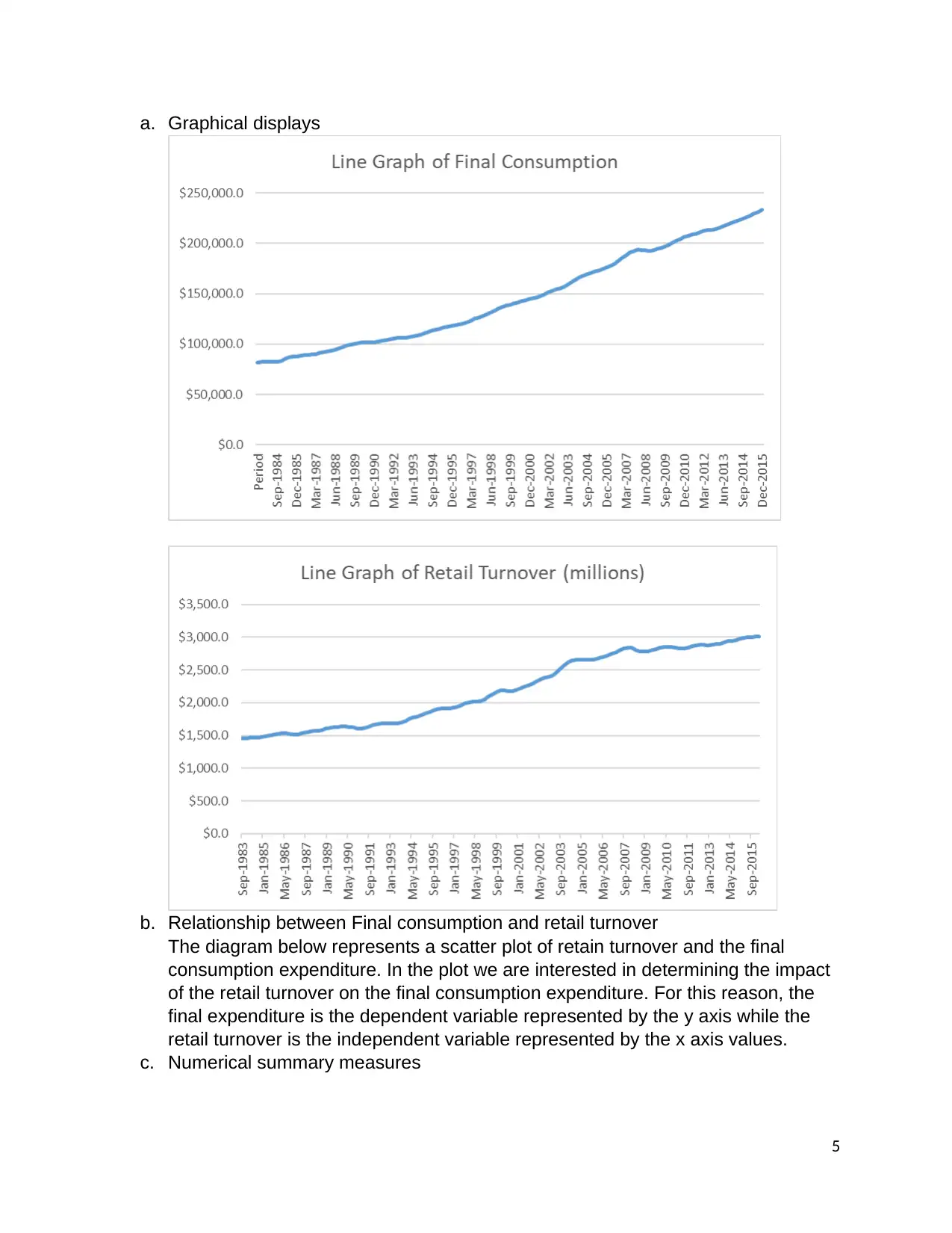
a. Graphical displays
b. Relationship between Final consumption and retail turnover
The diagram below represents a scatter plot of retain turnover and the final
consumption expenditure. In the plot we are interested in determining the impact
of the retail turnover on the final consumption expenditure. For this reason, the
final expenditure is the dependent variable represented by the y axis while the
retail turnover is the independent variable represented by the x axis values.
c. Numerical summary measures
5

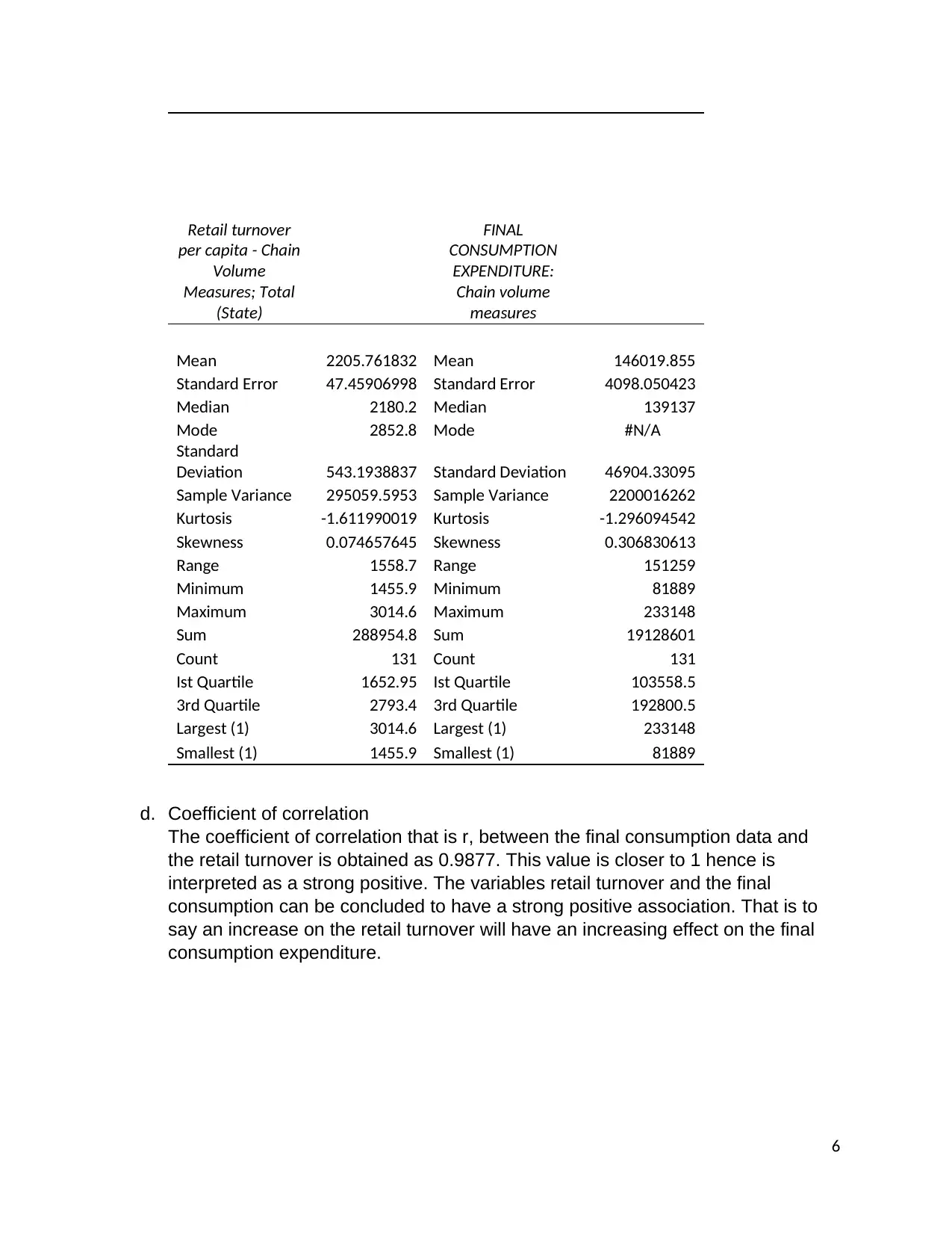
Retail turnover
per capita - Chain
Volume
Measures; Total
(State)
FINAL
CONSUMPTION
EXPENDITURE:
Chain volume
measures
Mean 2205.761832 Mean 146019.855
Standard Error 47.45906998 Standard Error 4098.050423
Median 2180.2 Median 139137
Mode 2852.8 Mode #N/A
Standard
Deviation 543.1938837 Standard Deviation 46904.33095
Sample Variance 295059.5953 Sample Variance 2200016262
Kurtosis -1.611990019 Kurtosis -1.296094542
Skewness 0.074657645 Skewness 0.306830613
Range 1558.7 Range 151259
Minimum 1455.9 Minimum 81889
Maximum 3014.6 Maximum 233148
Sum 288954.8 Sum 19128601
Count 131 Count 131
Ist Quartile 1652.95 Ist Quartile 103558.5
3rd Quartile 2793.4 3rd Quartile 192800.5
Largest (1) 3014.6 Largest (1) 233148
Smallest (1) 1455.9 Smallest (1) 81889
d. Coefficient of correlation
The coefficient of correlation that is r, between the final consumption data and
the retail turnover is obtained as 0.9877. This value is closer to 1 hence is
interpreted as a strong positive. The variables retail turnover and the final
consumption can be concluded to have a strong positive association. That is to
say an increase on the retail turnover will have an increasing effect on the final
consumption expenditure.
6

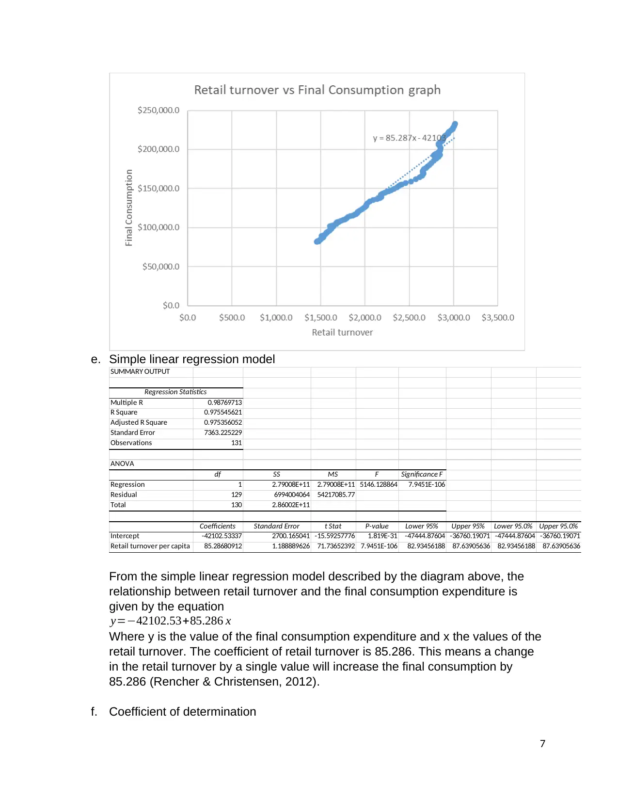
e. Simple linear regression model
SUMMARY OUTPUT
Regression Statistics
Multiple R 0.98769713
R Square 0.975545621
Adjusted R Square 0.975356052
Standard Error 7363.225229
Observations 131
ANOVA
df SS MS F Significance F
Regression 1 2.79008E+11 2.79008E+11 5146.128864 7.9451E-106
Residual 129 6994004064 54217085.77
Total 130 2.86002E+11
Coefficients Standard Error t Stat P-value Lower 95% Upper 95% Lower 95.0% Upper 95.0%
Intercept -42102.53337 2700.165041 -15.59257776 1.819E-31 -47444.87604 -36760.19071 -47444.87604 -36760.19071
Retail turnover per capita 85.28680912 1.188889626 71.73652392 7.9451E-106 82.93456188 87.63905636 82.93456188 87.63905636
From the simple linear regression model described by the diagram above, the
relationship between retail turnover and the final consumption expenditure is
given by the equation
y=−42102.53+85.286 x
Where y is the value of the final consumption expenditure and x the values of the
retail turnover. The coefficient of retail turnover is 85.286. This means a change
in the retail turnover by a single value will increase the final consumption by
85.286 (Rencher & Christensen, 2012).
f. Coefficient of determination
7

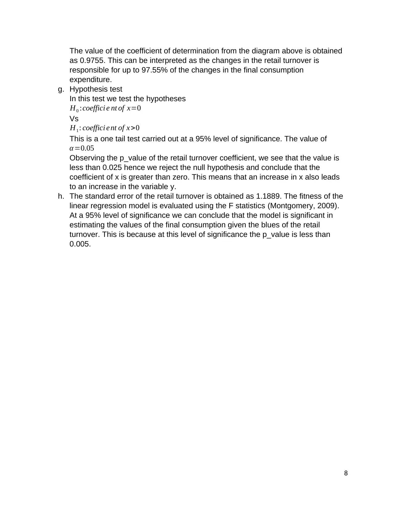
The value of the coefficient of determination from the diagram above is obtained
as 0.9755. This can be interpreted as the changes in the retail turnover is
responsible for up to 97.55% of the changes in the final consumption
expenditure.
g. Hypothesis test
In this test we test the hypotheses
H0 :coeffici e nt of x=0
Vs
H1 : coeffici e nt of x >0
This is a one tail test carried out at a 95% level of significance. The value of
α=0.05
Observing the p_value of the retail turnover coefficient, we see that the value is
less than 0.025 hence we reject the null hypothesis and conclude that the
coefficient of x is greater than zero. This means that an increase in x also leads
to an increase in the variable y.
h. The standard error of the retail turnover is obtained as 1.1889. The fitness of the
linear regression model is evaluated using the F statistics (Montgomery, 2009).
At a 95% level of significance we can conclude that the model is significant in
estimating the values of the final consumption given the blues of the retail
turnover. This is because at this level of significance the p_value is less than
0.005.
8

References
Montgomery, D., 2009. Design and analysis of experiments. , Hoboken, N.J.: Wiley.
Rencher, A. C. & Christensen, W. F., 2012. Methods of Multivariate Analysis; Wiley Series in Probability
and Statistics. 3rd ed. s.l.:John Wiley & Sons.
9