Statistics Assessment 1 for STA101 - Statistics for Business

This assessment covers topics like sample covariance, exponential distribution, power of test, rejection region, and more. It is relevant for students of STA101 - Statistics for Business.

Statistics Assessment 1
Unit: STA101 – Statistics for Business

Answer 1:
a. Sample Covariance between the variables is calculated as COV ( x , y ) =
∑
i =1
n
( xi −x
−
)( yi− y
−
)
n−1 where x
−
and y
−
are the sample means
x
−
= 5+3+7+ 9+2+4 +6+ 8
8 =5. 5
y
−
=20+23+15+11+27+21+17+14
8 =18 . 5
Table 1: Covariance Calculation Table
Observation x y Xi-X-bar Yi-Ybar (Xi-X-bar)^2 (Yi-Ybar)^2 (Xi-X-bar)*(Yi-Ybar)
1 5 20 -0.5 1.5 0.25 2.25 -0.75
2 3 23 -2.5 4.5 6.25 20.25 -11.25
3 7 15 1.5 -3.5 2.25 12.25 -5.25
4 9 11 3.5 -7.5 12.25 56.25 -26.25
5 2 27 -3.5 8.5 12.25 72.25 -29.75
6 4 21 -1.5 2.5 2.25 6.25 -3.75
7 6 17 0.5 -1.5 0.25 2.25 -0.75
8 8 14 2.5 -4.5 6.25 20.25 -11.25
Total 44 148 0 0 42 192 -89
Hence, sample covariance is calculated as COV ( x , y ) =−89
7 =−12 . 71
The covariance interpreted that the two variables had negative linear relation. This indicated that for
increase in X, Y would decrease linearly, and their directions are opposite (Puccio, Piilo, and

Tumminello, 2016).
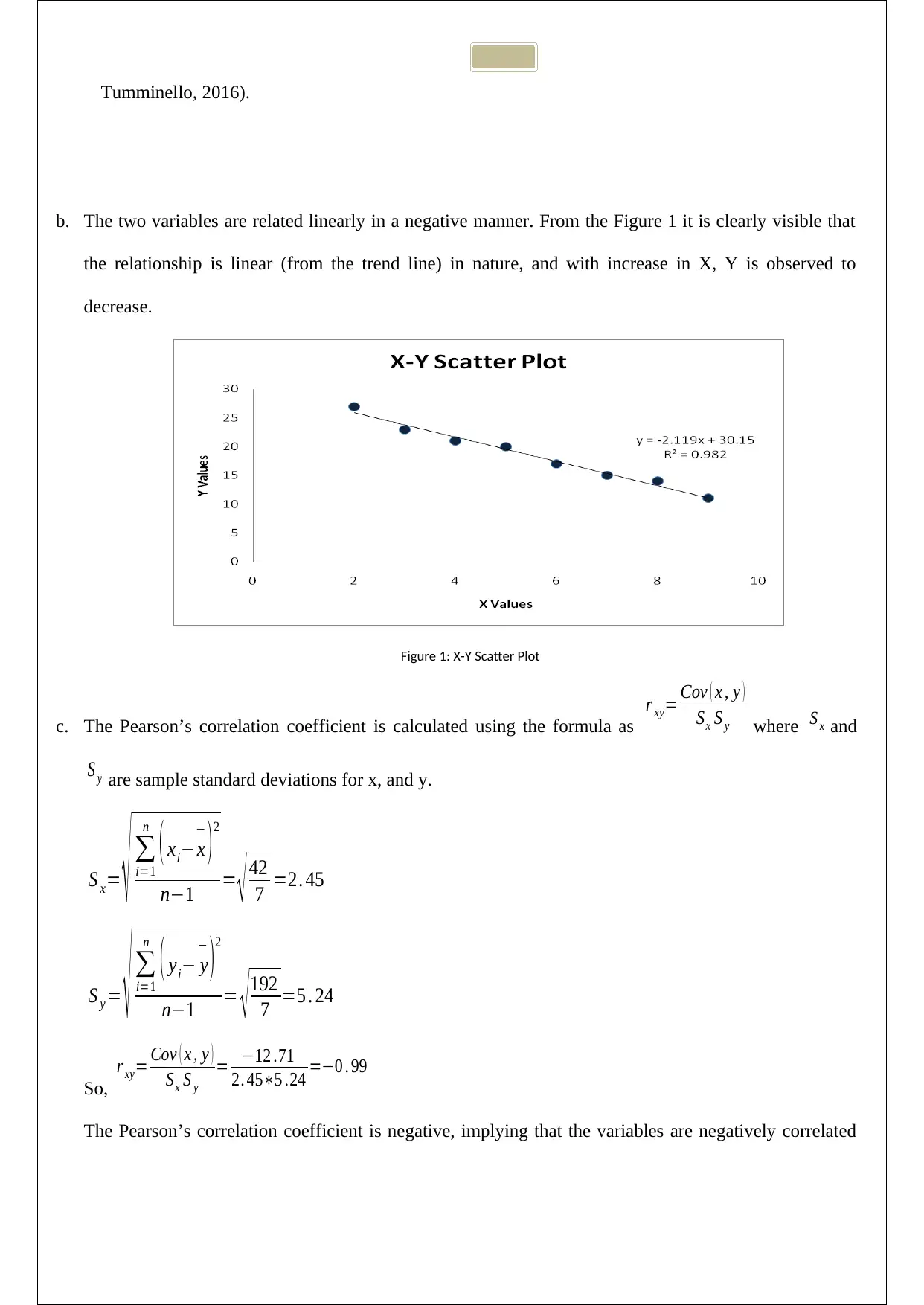
b. The two variables are related linearly in a negative manner. From the Figure 1 it is clearly visible that
the relationship is linear (from the trend line) in nature, and with increase in X, Y is observed to
decrease.
Figure 1: X-Y Scatter Plot
c. The Pearson’s correlation coefficient is calculated using the formula as
r xy= Cov ( x , y )
Sx S y where S x and
S y are sample standard deviations for x, and y.
S x= √ ∑
i=1
n
( xi−x
−
)
2
n−1 = √ 42
7 =2. 45
S y = √ ∑
i=1
n
( yi− y
−
)
2
n−1 = √ 192
7 =5 . 24
So,
r xy= Cov ( x , y )
Sx S y
= −12 .71
2. 45∗5 .24 =−0 . 99
The Pearson’s correlation coefficient is negative, implying that the variables are negatively correlated

with a high correlation (Cohen, West, and Aiken, 2014).
d. The trend of the relation of X and Y is clear from the scatter plot, where Y is decreasing for increase in
X. Hence, the negative value of the correlation is just an inferential conclusion to the negative linear
trend of the scatter plot data points.
a. For an exponential distribution, Mean or Average = E ( X ) = 1
λ where λ is the parameter of the
distribution. Hence, the rate parameter is λ= 1
mean= 1
3
b. Let the random variable X denotes the time customers willing to wait before ordering. Here X ~ exp ( λ )
and probability of waiting for more than 1.5 minutes is calculated as
P ( x ≥1. 5 ) = ∫
x=1 .5
∞
λe−λx dx
.
Now,
P ( x ≥1. 5 ) = ∫
x=1 .5
∞
λe−λx dx=1−P ( x <1 .5 ) =e
−1. 5
3=e−0 . 5=0 .606
Hence, probability of not wanting to wait more than 1.5 minutes = 1 – 0.606 = 0.394
Hence, in 39.4% cases people are hanging up before placing an order, if they have to wait after 1.5
minutes.
c. According to the problem, P ( x >T ) =0 . 1 where T is the required waiting time.
Now, P ( x >T ) =e− λT =0 . 1

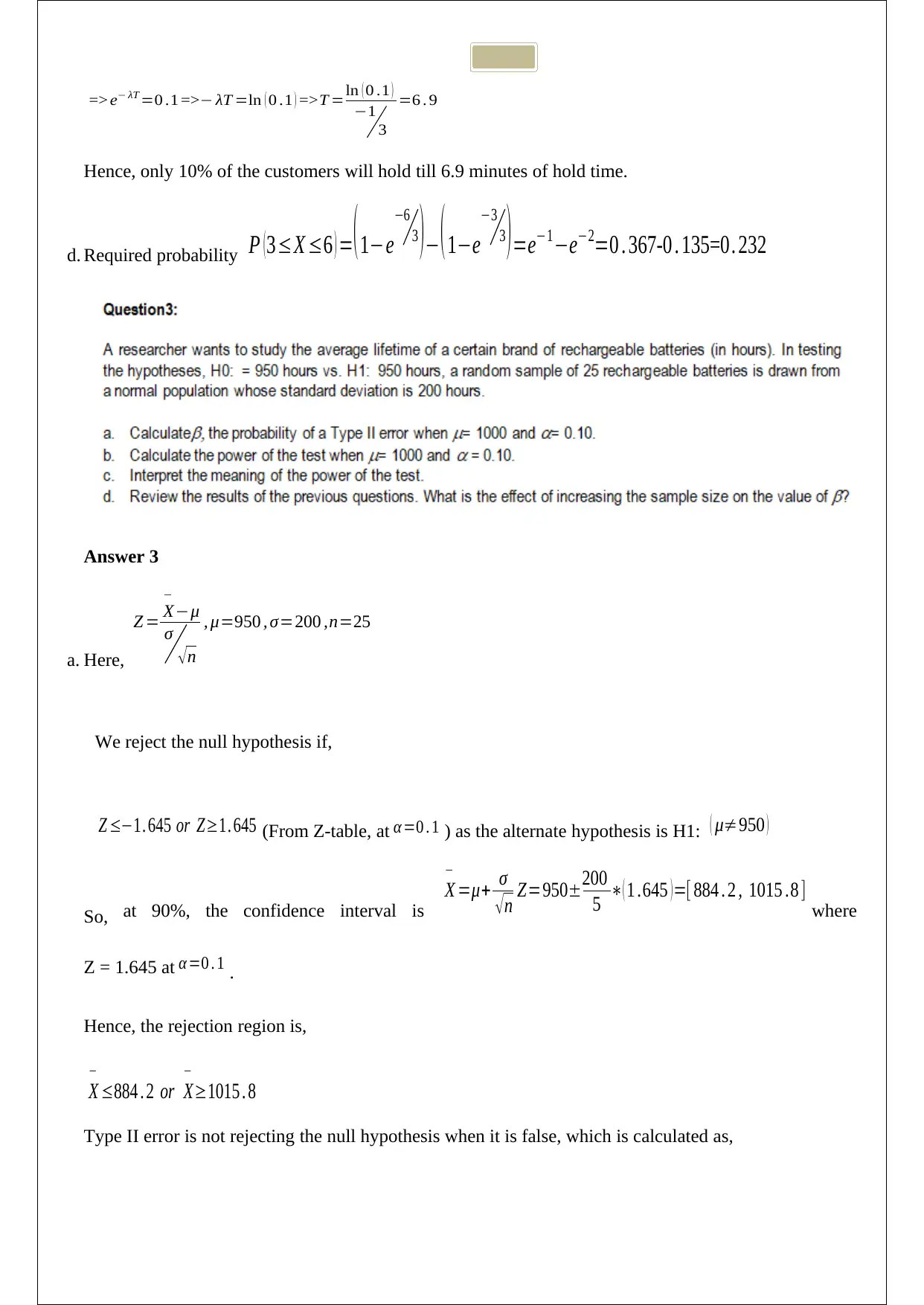
=> e− λT =0 .1 =>− λT =ln ( 0 .1 ) =>T =ln ( 0 .1 )
−1
3
=6 . 9
Hence, only 10% of the customers will hold till 6.9 minutes of hold time.
d. Required probability P ( 3≤X ≤6 ) =( 1−e
−6
3 )− ( 1−e
−3
3 ) =e−1−e−2=0 . 367-0 . 135=0. 232
Answer 3
a. Here,
Z = X
−
−μ
σ
√ n
, μ=950 , σ=200 ,n=25
We reject the null hypothesis if,
Z ≤−1. 645 or Z≥1. 645 (From Z-table, at α =0 . 1 ) as the alternate hypothesis is H1: ( μ≠950 )
So, at 90%, the confidence interval is
X
−
=μ+ σ
√ n Z=950±200
5 ∗( 1 .645 ) =[ 884 . 2 , 1015 .8 ] where
Z = 1.645 at α =0 . 1 .
Hence, the rejection region is,
X
−
≤884 . 2 or X
−
≥1015 . 8
Type II error is not rejecting the null hypothesis when it is false, which is calculated as,

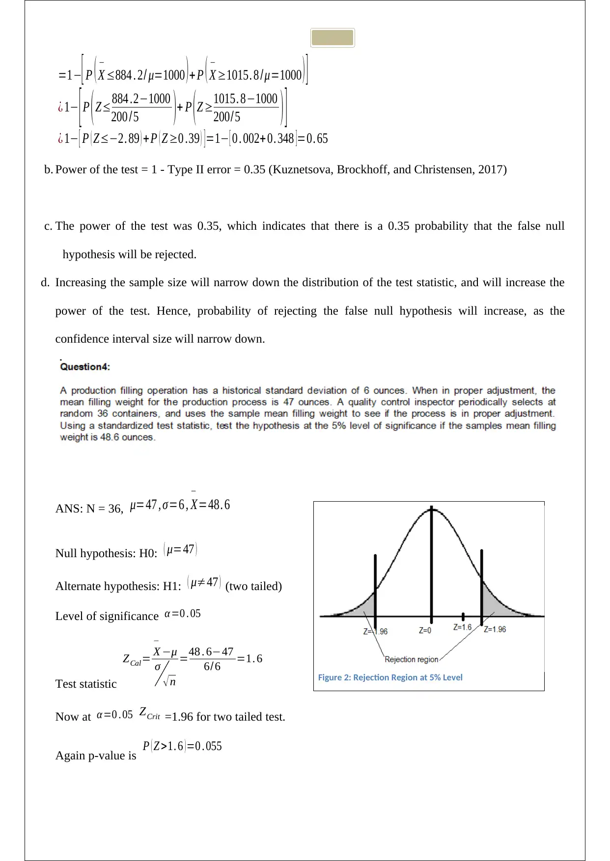
=1−[ P ( X
−
≤884 . 2/ μ=1000 ) + P ( X
−
≥1015. 8 /μ=1000 ) ]
¿ 1− [ P ( Z≤884 .2−1000
200 / 5 )+ P ( Z ≥1015. 8−1000
200/ 5 ) ]
¿ 1− [ P ( Z≤−2. 89 ) + P ( Z ≥0 .39 ) ] =1− [ 0 . 002+ 0. 348 ]=0. 65
b. Power of the test = 1 - Type II error = 0.35 (Kuznetsova, Brockhoff, and Christensen, 2017)
c. The power of the test was 0.35, which indicates that there is a 0.35 probability that the false null
hypothesis will be rejected.
d. Increasing the sample size will narrow down the distribution of the test statistic, and will increase the
power of the test. Hence, probability of rejecting the false null hypothesis will increase, as the
confidence interval size will narrow down.
ANS: N = 36, μ=47 , σ=6 , X
−
=48. 6
Null hypothesis: H0: ( μ=47 )
Alternate hypothesis: H1: ( μ≠47 ) (two tailed)
Level of significance α=0 . 05
Test statistic
ZCal= X
−
−μ
σ
√ n
=48 . 6−47
6/ 6 =1. 6
Now at α=0 . 05 ZCrit =1.96 for two tailed test.
Again p-value is P ( Z >1. 6 ) =0 . 055
Figure 2: Rejection Region at 5% Level

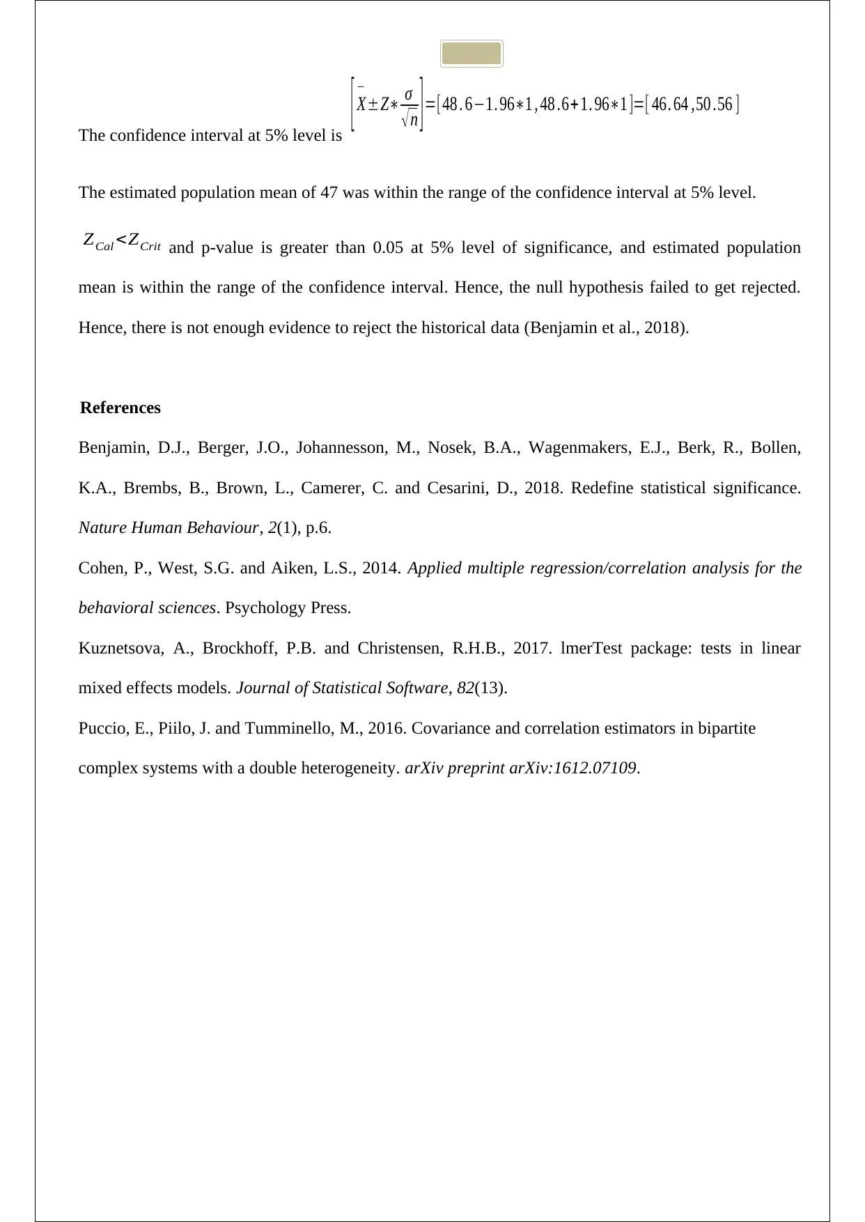
The confidence interval at 5% level is
[ X
−
±Z∗ σ
√ n ] =[48 . 6−1. 96∗1 , 48 .6+ 1. 96∗1 ]=[ 46. 64 ,50 .56 ]
The estimated population mean of 47 was within the range of the confidence interval at 5% level.
ZCal <ZCrit and p-value is greater than 0.05 at 5% level of significance, and estimated population
mean is within the range of the confidence interval. Hence, the null hypothesis failed to get rejected.
Hence, there is not enough evidence to reject the historical data (Benjamin et al., 2018).
References
Benjamin, D.J., Berger, J.O., Johannesson, M., Nosek, B.A., Wagenmakers, E.J., Berk, R., Bollen,
K.A., Brembs, B., Brown, L., Camerer, C. and Cesarini, D., 2018. Redefine statistical significance.
Nature Human Behaviour, 2(1), p.6.
Cohen, P., West, S.G. and Aiken, L.S., 2014. Applied multiple regression/correlation analysis for the
behavioral sciences. Psychology Press.
Kuznetsova, A., Brockhoff, P.B. and Christensen, R.H.B., 2017. lmerTest package: tests in linear
mixed effects models. Journal of Statistical Software, 82(13).
Puccio, E., Piilo, J. and Tumminello, M., 2016. Covariance and correlation estimators in bipartite
complex systems with a double heterogeneity. arXiv preprint arXiv:1612.07109.