Statistics Assignment: Analysis of Household Income and Expenses
VerifiedAdded on 2022/09/09
|12
|2071
|17
Homework Assignment
AI Summary
This statistics assignment analyzes household income, expenses, and related variables using descriptive statistics and data visualization. The assignment begins with generating a random sample of 200 households from a larger dataset, following a specific random sampling procedure. The student then calculates and interprets descriptive statistics such as mean, median, standard deviation, skewness, and kurtosis for various income and expenditure variables, including annual taxable income, total expenditure, and expenses on meals and clothing. Histograms are created to visualize the distributions of these variables, and the student comments on the skewness of the distributions. The analysis is performed separately for male and female heads of households, comparing income and expenditure patterns. Finally, the assignment examines the relationship between household size and homeownership, as well as the relationship between grocery expenses and eating-out expenses, including the calculation and interpretation of the R-squared statistic. The student provides tables, figures, and detailed interpretations throughout the analysis, referencing statistical concepts and providing insights into the data.
Running Head: STATISTICS ASSIGNMENT
Statistics Assignment
Name of the Student
Name of the University
Author Note
Statistics Assignment
Name of the Student
Name of the University
Author Note
Paraphrase This Document
Need a fresh take? Get an instant paraphrase of this document with our AI Paraphraser
1STATISTICS ASSIGNMENT
Table of Contents
Task 2.........................................................................................................................................2
Part A.....................................................................................................................................2
Part B......................................................................................................................................2
Part C......................................................................................................................................4
Part D.....................................................................................................................................4
Part E......................................................................................................................................6
Part F......................................................................................................................................6
Task 3.........................................................................................................................................7
Part A.....................................................................................................................................7
Part B......................................................................................................................................7
Part C......................................................................................................................................8
Part D.....................................................................................................................................8
Part E......................................................................................................................................8
Task 4.........................................................................................................................................8
Part A.....................................................................................................................................8
Part B......................................................................................................................................9
Part C......................................................................................................................................9
2STATISTICS ASSIGNMENT
Task 2
Part A
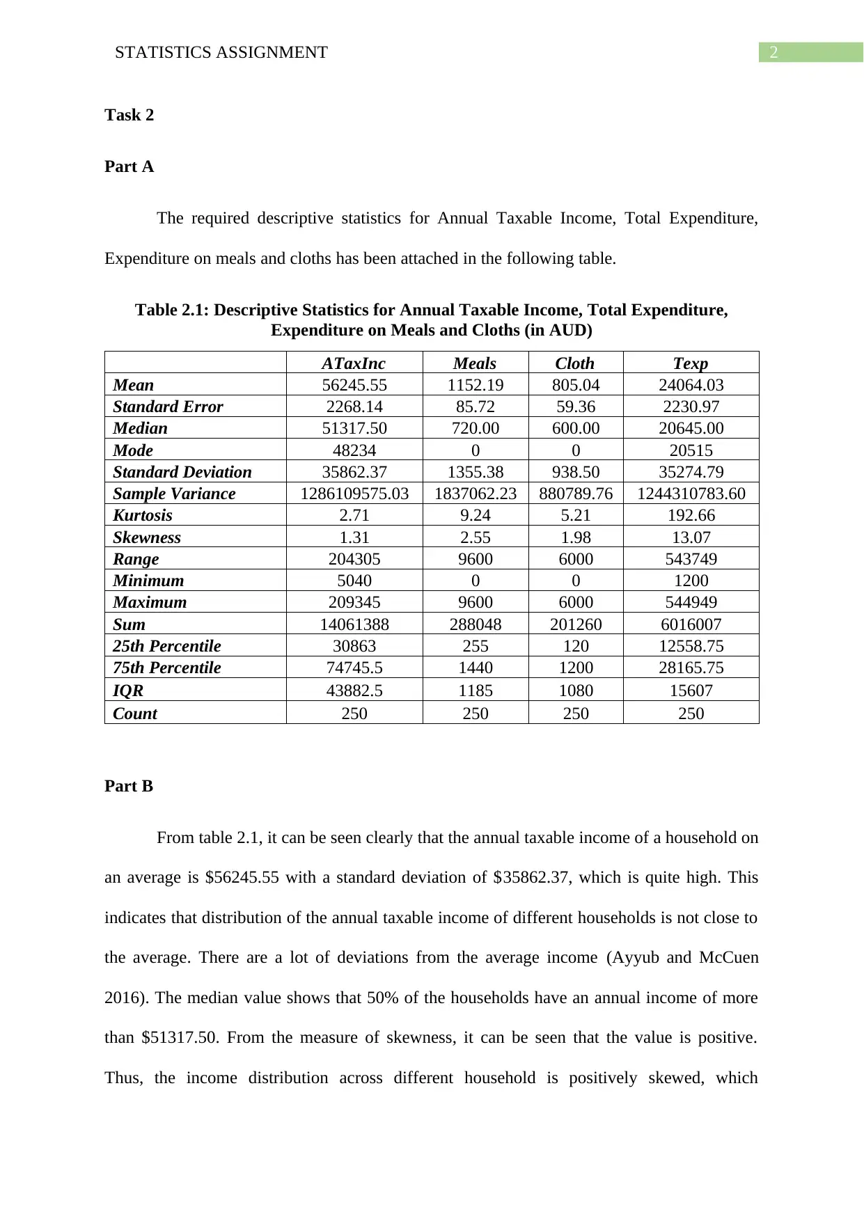
The required descriptive statistics for Annual Taxable Income, Total Expenditure,
Expenditure on meals and cloths has been attached in the following table.
Table 2.1: Descriptive Statistics for Annual Taxable Income, Total Expenditure,
Expenditure on Meals and Cloths (in AUD)
ATaxInc Meals Cloth Texp
Mean 56245.55 1152.19 805.04 24064.03
Standard Error 2268.14 85.72 59.36 2230.97
Median 51317.50 720.00 600.00 20645.00
Mode 48234 0 0 20515
Standard Deviation 35862.37 1355.38 938.50 35274.79
Sample Variance 1286109575.03 1837062.23 880789.76 1244310783.60
Kurtosis 2.71 9.24 5.21 192.66
Skewness 1.31 2.55 1.98 13.07
Range 204305 9600 6000 543749
Minimum 5040 0 0 1200
Maximum 209345 9600 6000 544949
Sum 14061388 288048 201260 6016007
25th Percentile 30863 255 120 12558.75
75th Percentile 74745.5 1440 1200 28165.75
IQR 43882.5 1185 1080 15607
Count 250 250 250 250
Part B
From table 2.1, it can be seen clearly that the annual taxable income of a household on
an average is $56245.55 with a standard deviation of $35862.37, which is quite high. This
indicates that distribution of the annual taxable income of different households is not close to
the average. There are a lot of deviations from the average income (Ayyub and McCuen
2016). The median value shows that 50% of the households have an annual income of more
than $51317.50. From the measure of skewness, it can be seen that the value is positive.
Thus, the income distribution across different household is positively skewed, which
Task 2
Part A
The required descriptive statistics for Annual Taxable Income, Total Expenditure,
Expenditure on meals and cloths has been attached in the following table.
Table 2.1: Descriptive Statistics for Annual Taxable Income, Total Expenditure,
Expenditure on Meals and Cloths (in AUD)
ATaxInc Meals Cloth Texp
Mean 56245.55 1152.19 805.04 24064.03
Standard Error 2268.14 85.72 59.36 2230.97
Median 51317.50 720.00 600.00 20645.00
Mode 48234 0 0 20515
Standard Deviation 35862.37 1355.38 938.50 35274.79
Sample Variance 1286109575.03 1837062.23 880789.76 1244310783.60
Kurtosis 2.71 9.24 5.21 192.66
Skewness 1.31 2.55 1.98 13.07
Range 204305 9600 6000 543749
Minimum 5040 0 0 1200
Maximum 209345 9600 6000 544949
Sum 14061388 288048 201260 6016007
25th Percentile 30863 255 120 12558.75
75th Percentile 74745.5 1440 1200 28165.75
IQR 43882.5 1185 1080 15607
Count 250 250 250 250
Part B
From table 2.1, it can be seen clearly that the annual taxable income of a household on
an average is $56245.55 with a standard deviation of $35862.37, which is quite high. This
indicates that distribution of the annual taxable income of different households is not close to
the average. There are a lot of deviations from the average income (Ayyub and McCuen
2016). The median value shows that 50% of the households have an annual income of more
than $51317.50. From the measure of skewness, it can be seen that the value is positive.
Thus, the income distribution across different household is positively skewed, which
⊘ This is a preview!⊘
Do you want full access?
Subscribe today to unlock all pages.
Trusted by 1+ million students worldwide
3STATISTICS ASSIGNMENT
indicates that there are higher number of households which have an annual income less than
the average annual income of the households.
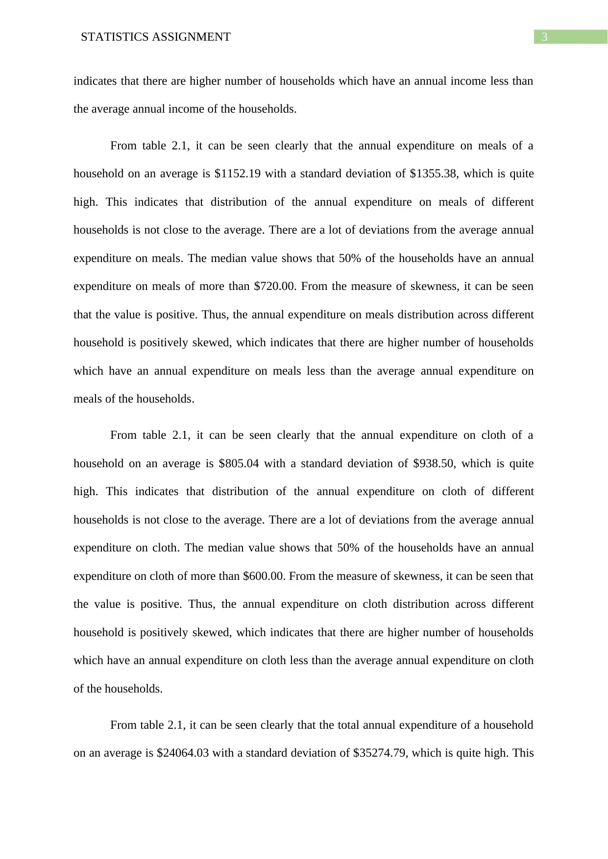
From table 2.1, it can be seen clearly that the annual expenditure on meals of a
household on an average is $1152.19 with a standard deviation of $1355.38, which is quite
high. This indicates that distribution of the annual expenditure on meals of different
households is not close to the average. There are a lot of deviations from the average annual
expenditure on meals. The median value shows that 50% of the households have an annual
expenditure on meals of more than $720.00. From the measure of skewness, it can be seen
that the value is positive. Thus, the annual expenditure on meals distribution across different
household is positively skewed, which indicates that there are higher number of households
which have an annual expenditure on meals less than the average annual expenditure on
meals of the households.
From table 2.1, it can be seen clearly that the annual expenditure on cloth of a
household on an average is $805.04 with a standard deviation of $938.50, which is quite
high. This indicates that distribution of the annual expenditure on cloth of different
households is not close to the average. There are a lot of deviations from the average annual
expenditure on cloth. The median value shows that 50% of the households have an annual
expenditure on cloth of more than $600.00. From the measure of skewness, it can be seen that
the value is positive. Thus, the annual expenditure on cloth distribution across different
household is positively skewed, which indicates that there are higher number of households
which have an annual expenditure on cloth less than the average annual expenditure on cloth
of the households.
From table 2.1, it can be seen clearly that the total annual expenditure of a household
on an average is $24064.03 with a standard deviation of $35274.79, which is quite high. This
indicates that there are higher number of households which have an annual income less than
the average annual income of the households.
From table 2.1, it can be seen clearly that the annual expenditure on meals of a
household on an average is $1152.19 with a standard deviation of $1355.38, which is quite
high. This indicates that distribution of the annual expenditure on meals of different
households is not close to the average. There are a lot of deviations from the average annual
expenditure on meals. The median value shows that 50% of the households have an annual
expenditure on meals of more than $720.00. From the measure of skewness, it can be seen
that the value is positive. Thus, the annual expenditure on meals distribution across different
household is positively skewed, which indicates that there are higher number of households
which have an annual expenditure on meals less than the average annual expenditure on
meals of the households.
From table 2.1, it can be seen clearly that the annual expenditure on cloth of a
household on an average is $805.04 with a standard deviation of $938.50, which is quite
high. This indicates that distribution of the annual expenditure on cloth of different
households is not close to the average. There are a lot of deviations from the average annual
expenditure on cloth. The median value shows that 50% of the households have an annual
expenditure on cloth of more than $600.00. From the measure of skewness, it can be seen that
the value is positive. Thus, the annual expenditure on cloth distribution across different
household is positively skewed, which indicates that there are higher number of households
which have an annual expenditure on cloth less than the average annual expenditure on cloth
of the households.
From table 2.1, it can be seen clearly that the total annual expenditure of a household
on an average is $24064.03 with a standard deviation of $35274.79, which is quite high. This
Paraphrase This Document
Need a fresh take? Get an instant paraphrase of this document with our AI Paraphraser
4STATISTICS ASSIGNMENT
indicates that distribution of the total annual expenditure of different households is not close
to the average. There are a lot of deviations from the average of the total annual expenditure.
The median value shows that 50% of the households have a total annual expenditure of more
than $20645.00. From the measure of skewness, it can be seen that the value is positive.
Thus, the distribution of total annual expenditure across different household is positively
skewed, which indicates that there are higher number of households which have a total
annual expenditure less than the average of total annual expenditure of the households.
Part C
From the descriptive statistics presented in table 2.1, it can be said clearly that the
distribution of the four variables considered are of the same type. Less number of households
earn more than the average income and hence the expenses are also less than the average
expenses for most of the households. Here, the expenses include expenses on clothes, meal
and total expenses.
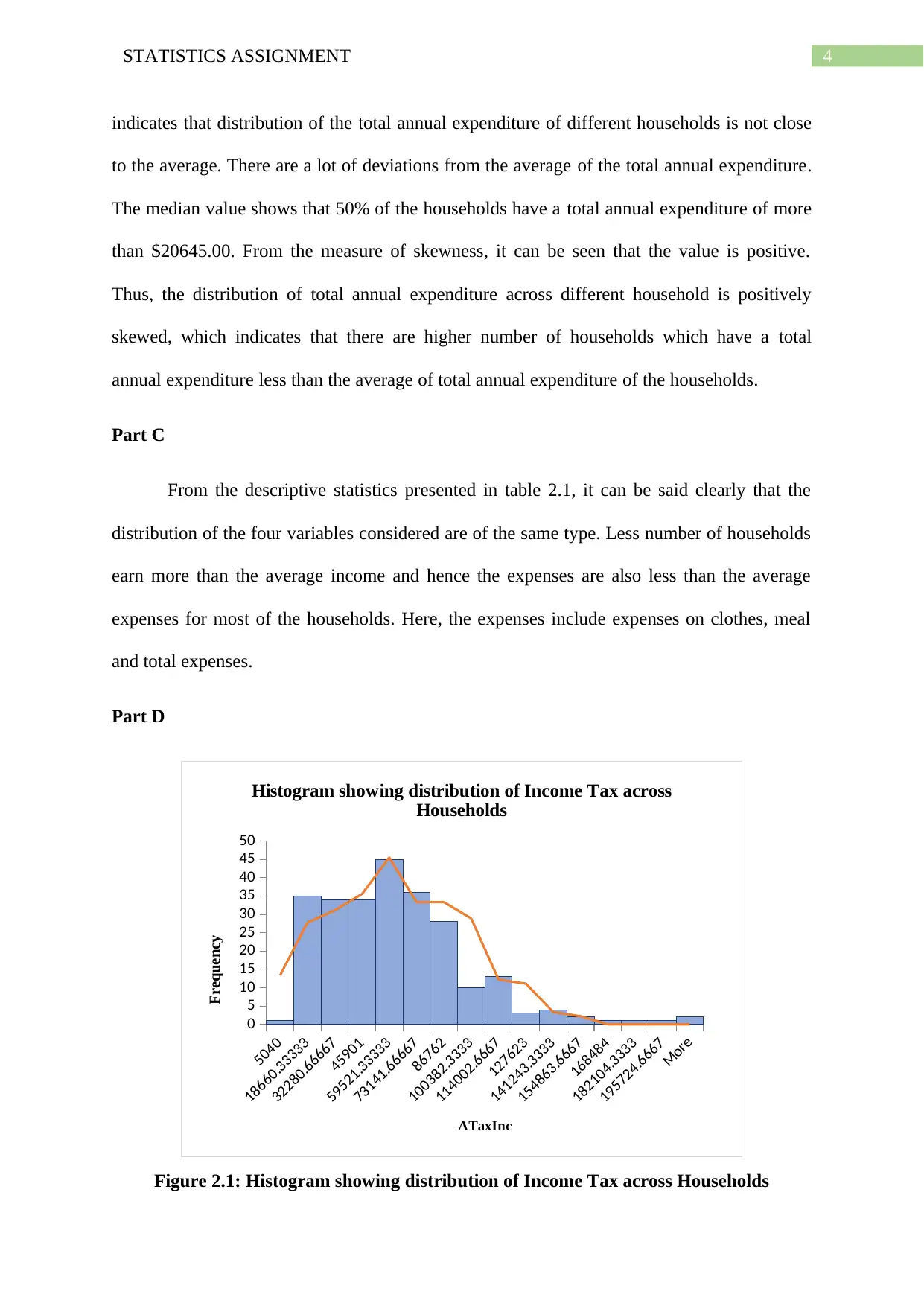
Part D
5040
18660.33333
32280.66667
45901
59521.33333
73141.66667
86762
100382.3333
114002.6667
127623
141243.3333
154863.6667
168484
182104.3333
195724.6667
More
0
5
10
15
20
25
30
35
40
45
50
0
5
10
15
20
25
30
35
40
45
Histogram showing distribution of Income Tax across
Households
ATaxInc
Frequency
Figure 2.1: Histogram showing distribution of Income Tax across Households
indicates that distribution of the total annual expenditure of different households is not close
to the average. There are a lot of deviations from the average of the total annual expenditure.
The median value shows that 50% of the households have a total annual expenditure of more
than $20645.00. From the measure of skewness, it can be seen that the value is positive.
Thus, the distribution of total annual expenditure across different household is positively
skewed, which indicates that there are higher number of households which have a total
annual expenditure less than the average of total annual expenditure of the households.
Part C
From the descriptive statistics presented in table 2.1, it can be said clearly that the
distribution of the four variables considered are of the same type. Less number of households
earn more than the average income and hence the expenses are also less than the average
expenses for most of the households. Here, the expenses include expenses on clothes, meal
and total expenses.
Part D
5040
18660.33333
32280.66667
45901
59521.33333
73141.66667
86762
100382.3333
114002.6667
127623
141243.3333
154863.6667
168484
182104.3333
195724.6667
More
0
5
10
15
20
25
30
35
40
45
50
0
5
10
15
20
25
30
35
40
45
Histogram showing distribution of Income Tax across
Households
ATaxInc
Frequency
Figure 2.1: Histogram showing distribution of Income Tax across Households
5STATISTICS ASSIGNMENT
0
640
1280
1920
2560
3200
3840
4480
5120
5760
6400
7040
7680
8320
8960
More
0
10
20
30
40
50
60
70
80
90
100
Histogram Showing Distribution of Meal Expenses
across Households
Meals
Frequency
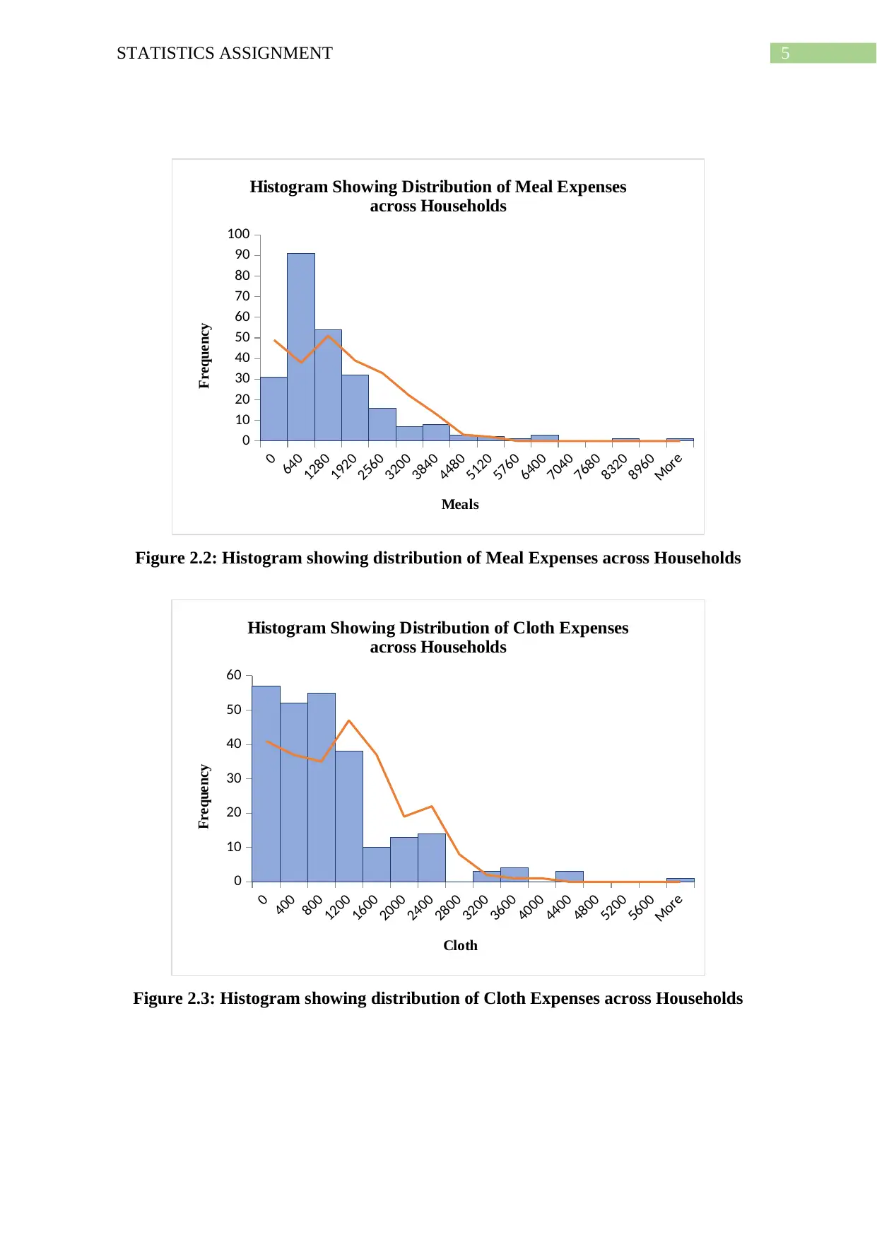
Figure 2.2: Histogram showing distribution of Meal Expenses across Households
0
400
800
1200
1600
2000
2400
2800
3200
3600
4000
4400
4800
5200
5600
More
0
10
20
30
40
50
60
Histogram Showing Distribution of Cloth Expenses
across Households
Cloth
Frequency
Figure 2.3: Histogram showing distribution of Cloth Expenses across Households
0
640
1280
1920
2560
3200
3840
4480
5120
5760
6400
7040
7680
8320
8960
More
0
10
20
30
40
50
60
70
80
90
100
Histogram Showing Distribution of Meal Expenses
across Households
Meals
Frequency
Figure 2.2: Histogram showing distribution of Meal Expenses across Households
0
400
800
1200
1600
2000
2400
2800
3200
3600
4000
4400
4800
5200
5600
More
0
10
20
30
40
50
60
Histogram Showing Distribution of Cloth Expenses
across Households
Cloth
Frequency
Figure 2.3: Histogram showing distribution of Cloth Expenses across Households
⊘ This is a preview!⊘
Do you want full access?
Subscribe today to unlock all pages.
Trusted by 1+ million students worldwide
6STATISTICS ASSIGNMENT
1200
37449.93333
73699.86667
109949.8
146199.7333
182449.6667
218699.6
254949.5333
291199.4667
327449.4
363699.3333
399949.2667
436199.2
472449.1333
508699.0667
More
0
50
100
150
200
250
0
10
20
30
40
50
60
70
80
90
100
Histogram Showing Distribution of Total Expenses
across Households
Texp
Frequency
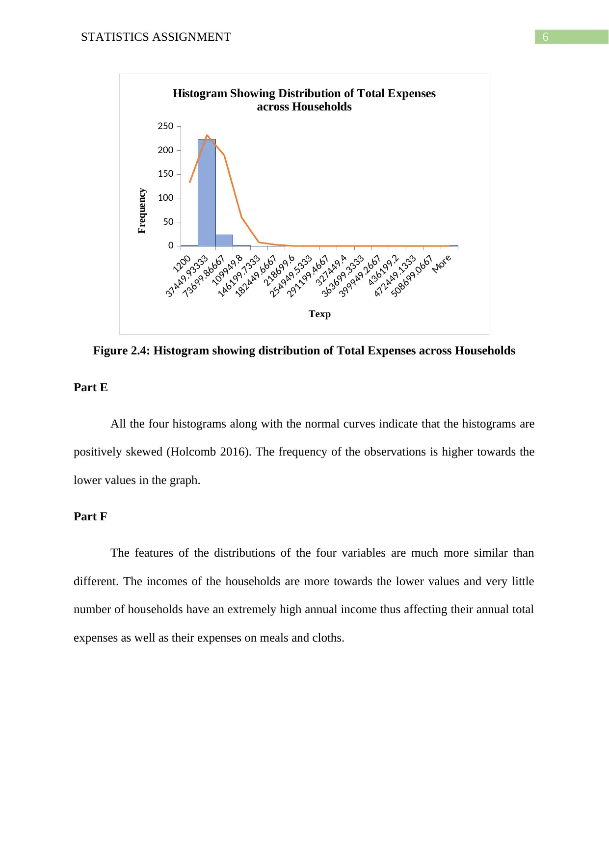
Figure 2.4: Histogram showing distribution of Total Expenses across Households
Part E
All the four histograms along with the normal curves indicate that the histograms are
positively skewed (Holcomb 2016). The frequency of the observations is higher towards the
lower values in the graph.
Part F
The features of the distributions of the four variables are much more similar than
different. The incomes of the households are more towards the lower values and very little
number of households have an extremely high annual income thus affecting their annual total
expenses as well as their expenses on meals and cloths.
1200
37449.93333
73699.86667
109949.8
146199.7333
182449.6667
218699.6
254949.5333
291199.4667
327449.4
363699.3333
399949.2667
436199.2
472449.1333
508699.0667
More
0
50
100
150
200
250
0
10
20
30
40
50
60
70
80
90
100
Histogram Showing Distribution of Total Expenses
across Households
Texp
Frequency
Figure 2.4: Histogram showing distribution of Total Expenses across Households
Part E
All the four histograms along with the normal curves indicate that the histograms are
positively skewed (Holcomb 2016). The frequency of the observations is higher towards the
lower values in the graph.
Part F
The features of the distributions of the four variables are much more similar than
different. The incomes of the households are more towards the lower values and very little
number of households have an extremely high annual income thus affecting their annual total
expenses as well as their expenses on meals and cloths.
Paraphrase This Document
Need a fresh take? Get an instant paraphrase of this document with our AI Paraphraser
7STATISTICS ASSIGNMENT
Task 3
Part A
The descriptive statistics for the four selected variables separately for males and
females are given in the following tables 3.1 and 3.2 respectively.
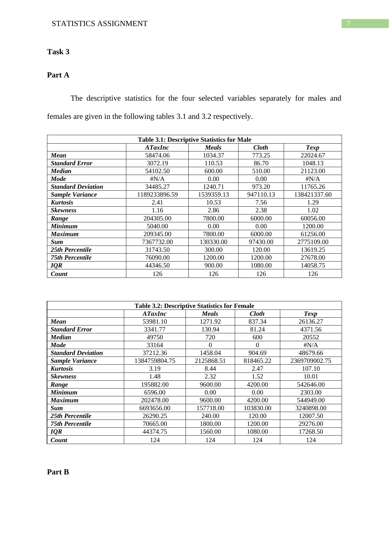
Table 3.1: Descriptive Statistics for Male
ATaxInc Meals Cloth Texp
Mean 58474.06 1034.37 773.25 22024.67
Standard Error 3072.19 110.53 86.70 1048.13
Median 54102.50 600.00 510.00 21123.00
Mode #N/A 0.00 0.00 #N/A
Standard Deviation 34485.27 1240.71 973.20 11765.26
Sample Variance 1189233896.59 1539359.13 947110.13 138421337.60
Kurtosis 2.41 10.53 7.56 1.29
Skewness 1.16 2.86 2.38 1.02
Range 204305.00 7800.00 6000.00 60056.00
Minimum 5040.00 0.00 0.00 1200.00
Maximum 209345.00 7800.00 6000.00 61256.00
Sum 7367732.00 130330.00 97430.00 2775109.00
25th Percentile 31743.50 300.00 120.00 13619.25
75th Percentile 76090.00 1200.00 1200.00 27678.00
IQR 44346.50 900.00 1080.00 14058.75
Count 126 126 126 126
Table 3.2: Descriptive Statistics for Female
ATaxInc Meals Cloth Texp
Mean 53981.10 1271.92 837.34 26136.27
Standard Error 3341.77 130.94 81.24 4371.56
Median 49750 720 600 20552
Mode 33164 0 0 #N/A
Standard Deviation 37212.36 1458.04 904.69 48679.66
Sample Variance 1384759804.75 2125868.51 818465.22 2369709002.75
Kurtosis 3.19 8.44 2.47 107.10
Skewness 1.48 2.32 1.52 10.01
Range 195882.00 9600.00 4200.00 542646.00
Minimum 6596.00 0.00 0.00 2303.00
Maximum 202478.00 9600.00 4200.00 544949.00
Sum 6693656.00 157718.00 103830.00 3240898.00
25th Percentile 26290.25 240.00 120.00 12007.50
75th Percentile 70665.00 1800.00 1200.00 29276.00
IQR 44374.75 1560.00 1080.00 17268.50
Count 124 124 124 124
Part B
Task 3
Part A
The descriptive statistics for the four selected variables separately for males and
females are given in the following tables 3.1 and 3.2 respectively.
Table 3.1: Descriptive Statistics for Male
ATaxInc Meals Cloth Texp
Mean 58474.06 1034.37 773.25 22024.67
Standard Error 3072.19 110.53 86.70 1048.13
Median 54102.50 600.00 510.00 21123.00
Mode #N/A 0.00 0.00 #N/A
Standard Deviation 34485.27 1240.71 973.20 11765.26
Sample Variance 1189233896.59 1539359.13 947110.13 138421337.60
Kurtosis 2.41 10.53 7.56 1.29
Skewness 1.16 2.86 2.38 1.02
Range 204305.00 7800.00 6000.00 60056.00
Minimum 5040.00 0.00 0.00 1200.00
Maximum 209345.00 7800.00 6000.00 61256.00
Sum 7367732.00 130330.00 97430.00 2775109.00
25th Percentile 31743.50 300.00 120.00 13619.25
75th Percentile 76090.00 1200.00 1200.00 27678.00
IQR 44346.50 900.00 1080.00 14058.75
Count 126 126 126 126
Table 3.2: Descriptive Statistics for Female
ATaxInc Meals Cloth Texp
Mean 53981.10 1271.92 837.34 26136.27
Standard Error 3341.77 130.94 81.24 4371.56
Median 49750 720 600 20552
Mode 33164 0 0 #N/A
Standard Deviation 37212.36 1458.04 904.69 48679.66
Sample Variance 1384759804.75 2125868.51 818465.22 2369709002.75
Kurtosis 3.19 8.44 2.47 107.10
Skewness 1.48 2.32 1.52 10.01
Range 195882.00 9600.00 4200.00 542646.00
Minimum 6596.00 0.00 0.00 2303.00
Maximum 202478.00 9600.00 4200.00 544949.00
Sum 6693656.00 157718.00 103830.00 3240898.00
25th Percentile 26290.25 240.00 120.00 12007.50
75th Percentile 70665.00 1800.00 1200.00 29276.00
IQR 44374.75 1560.00 1080.00 17268.50
Count 124 124 124 124
Part B
8STATISTICS ASSIGNMENT
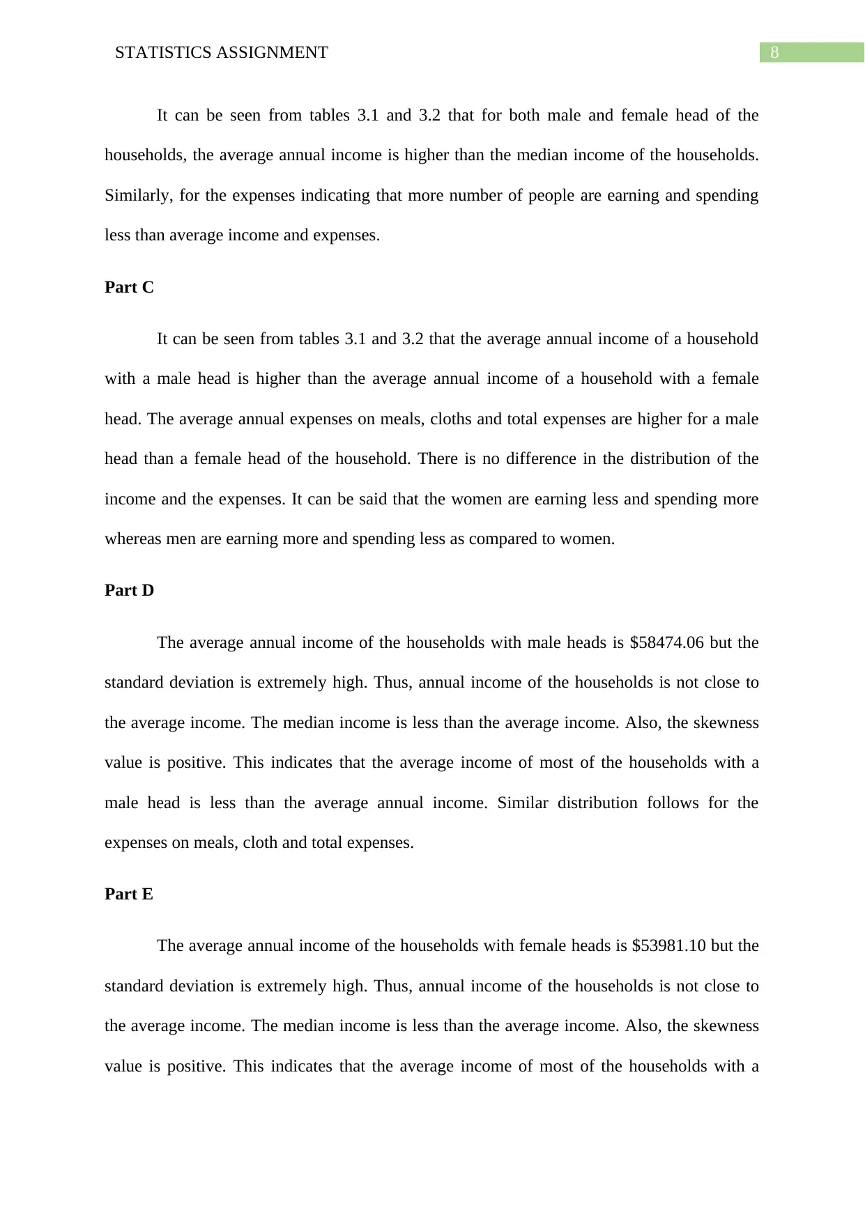
It can be seen from tables 3.1 and 3.2 that for both male and female head of the
households, the average annual income is higher than the median income of the households.
Similarly, for the expenses indicating that more number of people are earning and spending
less than average income and expenses.
Part C
It can be seen from tables 3.1 and 3.2 that the average annual income of a household
with a male head is higher than the average annual income of a household with a female
head. The average annual expenses on meals, cloths and total expenses are higher for a male
head than a female head of the household. There is no difference in the distribution of the
income and the expenses. It can be said that the women are earning less and spending more
whereas men are earning more and spending less as compared to women.
Part D
The average annual income of the households with male heads is $58474.06 but the
standard deviation is extremely high. Thus, annual income of the households is not close to
the average income. The median income is less than the average income. Also, the skewness
value is positive. This indicates that the average income of most of the households with a
male head is less than the average annual income. Similar distribution follows for the
expenses on meals, cloth and total expenses.
Part E
The average annual income of the households with female heads is $53981.10 but the
standard deviation is extremely high. Thus, annual income of the households is not close to
the average income. The median income is less than the average income. Also, the skewness
value is positive. This indicates that the average income of most of the households with a
⊘ This is a preview!⊘
Do you want full access?
Subscribe today to unlock all pages.
Trusted by 1+ million students worldwide
9STATISTICS ASSIGNMENT
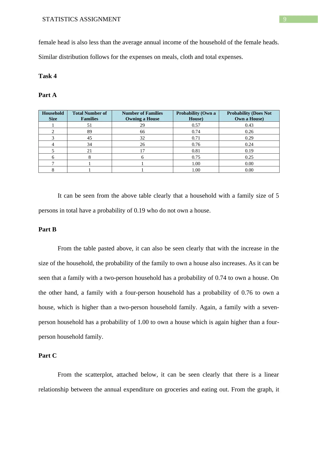
female head is also less than the average annual income of the household of the female heads.
Similar distribution follows for the expenses on meals, cloth and total expenses.
Task 4
Part A
Household
Size
Total Number of
Families
Number of Families
Owning a House
Probability (Own a
House)
Probability (Does Not
Own a House)
1 51 29 0.57 0.43
2 89 66 0.74 0.26
3 45 32 0.71 0.29
4 34 26 0.76 0.24
5 21 17 0.81 0.19
6 8 6 0.75 0.25
7 1 1 1.00 0.00
8 1 1 1.00 0.00
It can be seen from the above table clearly that a household with a family size of 5
persons in total have a probability of 0.19 who do not own a house.
Part B
From the table pasted above, it can also be seen clearly that with the increase in the
size of the household, the probability of the family to own a house also increases. As it can be
seen that a family with a two-person household has a probability of 0.74 to own a house. On
the other hand, a family with a four-person household has a probability of 0.76 to own a
house, which is higher than a two-person household family. Again, a family with a seven-
person household has a probability of 1.00 to own a house which is again higher than a four-
person household family.
Part C
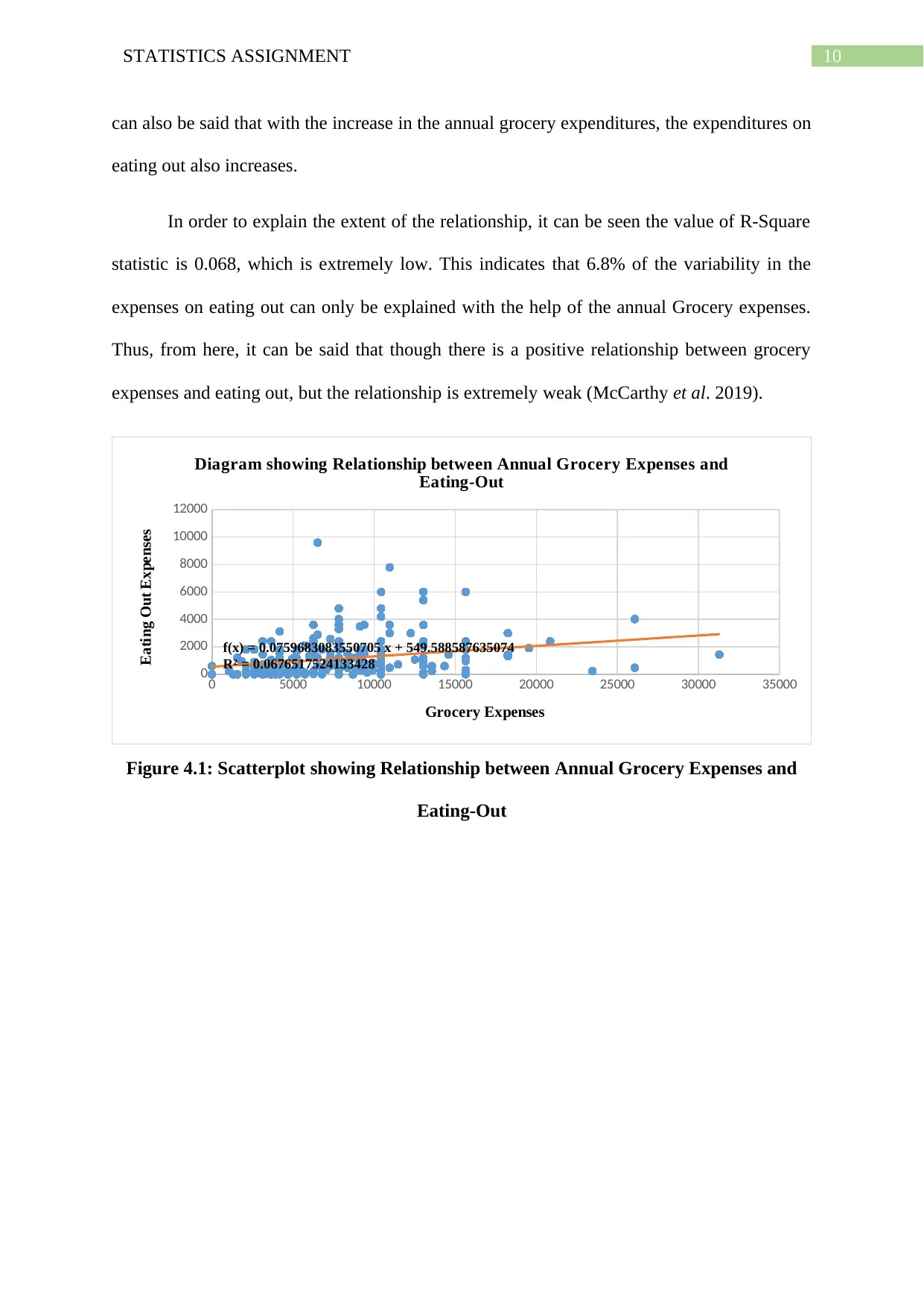
From the scatterplot, attached below, it can be seen clearly that there is a linear
relationship between the annual expenditure on groceries and eating out. From the graph, it
female head is also less than the average annual income of the household of the female heads.
Similar distribution follows for the expenses on meals, cloth and total expenses.
Task 4
Part A
Household
Size
Total Number of
Families
Number of Families
Owning a House
Probability (Own a
House)
Probability (Does Not
Own a House)
1 51 29 0.57 0.43
2 89 66 0.74 0.26
3 45 32 0.71 0.29
4 34 26 0.76 0.24
5 21 17 0.81 0.19
6 8 6 0.75 0.25
7 1 1 1.00 0.00
8 1 1 1.00 0.00
It can be seen from the above table clearly that a household with a family size of 5
persons in total have a probability of 0.19 who do not own a house.
Part B
From the table pasted above, it can also be seen clearly that with the increase in the
size of the household, the probability of the family to own a house also increases. As it can be
seen that a family with a two-person household has a probability of 0.74 to own a house. On
the other hand, a family with a four-person household has a probability of 0.76 to own a
house, which is higher than a two-person household family. Again, a family with a seven-
person household has a probability of 1.00 to own a house which is again higher than a four-
person household family.
Part C
From the scatterplot, attached below, it can be seen clearly that there is a linear
relationship between the annual expenditure on groceries and eating out. From the graph, it
Paraphrase This Document
Need a fresh take? Get an instant paraphrase of this document with our AI Paraphraser
10STATISTICS ASSIGNMENT
can also be said that with the increase in the annual grocery expenditures, the expenditures on
eating out also increases.
In order to explain the extent of the relationship, it can be seen the value of R-Square
statistic is 0.068, which is extremely low. This indicates that 6.8% of the variability in the
expenses on eating out can only be explained with the help of the annual Grocery expenses.
Thus, from here, it can be said that though there is a positive relationship between grocery
expenses and eating out, but the relationship is extremely weak (McCarthy et al. 2019).
0 5000 10000 15000 20000 25000 30000 35000
0
2000
4000
6000
8000
10000
12000
f(x) = 0.0759683083550705 x + 549.588587635074
R² = 0.0676517524133428
Diagram showing Relationship between Annual Grocery Expenses and
Eating-Out
Grocery Expenses
Eating Out Expenses
Figure 4.1: Scatterplot showing Relationship between Annual Grocery Expenses and
Eating-Out
11STATISTICS ASSIGNMENT
References
Ayyub, B.M. and McCuen, R.H., 2016. Probability, statistics, and reliability for engineers
and scientists. New York: CRC press.
Holcomb, Z.C., 2016. Fundamentals of descriptive statistics. New York: Routledge.
McCarthy, R.V., McCarthy, M.M., Ceccucci, W. and Halawi, L., 2019. What Do Descriptive
Statistics Tell Us. In Applying Predictive Analytics (pp. 57-87). Switzerland: Springer, Cham.
⊘ This is a preview!⊘
Do you want full access?
Subscribe today to unlock all pages.
Trusted by 1+ million students worldwide
1 out of 12
Related Documents


Your All-in-One AI-Powered Toolkit for Academic Success.
+13062052269
info@desklib.com
Available 24*7 on WhatsApp / Email
![[object Object]](/_next/static/media/star-bottom.7253800d.svg)
Unlock your academic potential
Copyright © 2020–2025 A2Z Services. All Rights Reserved. Developed and managed by ZUCOL.