Statistics Assignment - Quantitative Data

Running head: THREE TASKS 1
Three Tasks
Name of Student
Institution Affiliation

STATISTICS ASSIGNMENT 2
Three Tasks
Introduction and summary
The data presented on the file “Survey_Data_Sem2.xls” presents data from a sample of
students highlighting their individual attributes and other aspects related to their stay and
educational activities in the university. The students are categorized according to their home
regions as United Kingdom, European Region or International students. The other personal data
that is included in the data includes the age of the students and their gender. The data highlights
data on the satisfaction of the students’ accommodation, time spent on technological equipment
such as computers, exercise, part time employment, and study of math. The data is therefore
highly exhaustive and enables anyone interested in it to determine the relationship of various
variables. Some of the descriptive statistics that can be considered in the data include the means,
the medians, modes, standard deviation as well as the number of various variables among others.
It is thus important to describe and analyze the data to come up with the appropriate
relationships.
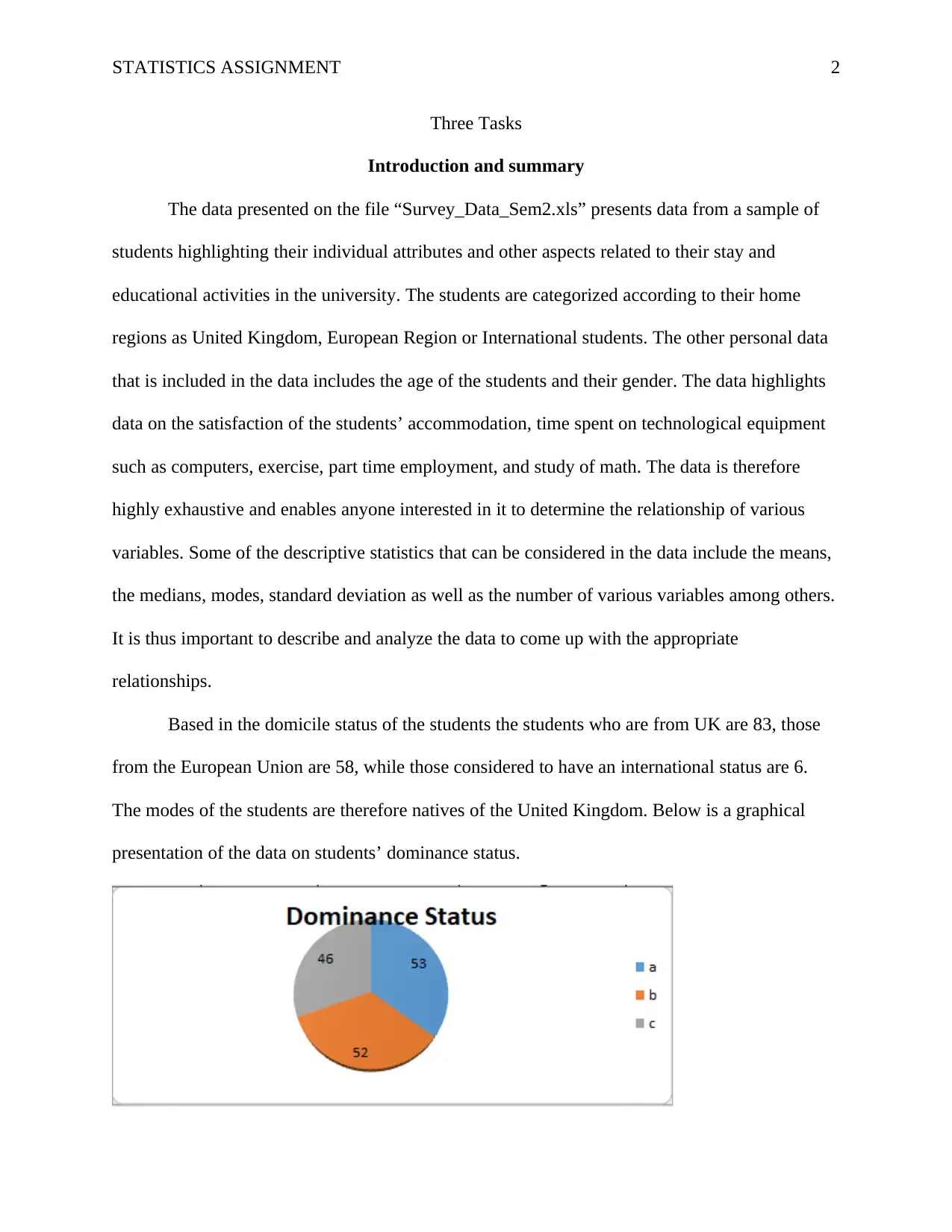
Based in the domicile status of the students the students who are from UK are 83, those
from the European Union are 58, while those considered to have an international status are 6.
The modes of the students are therefore natives of the United Kingdom. Below is a graphical
presentation of the data on students’ dominance status.

STATISTICS ASSIGNMENT 3
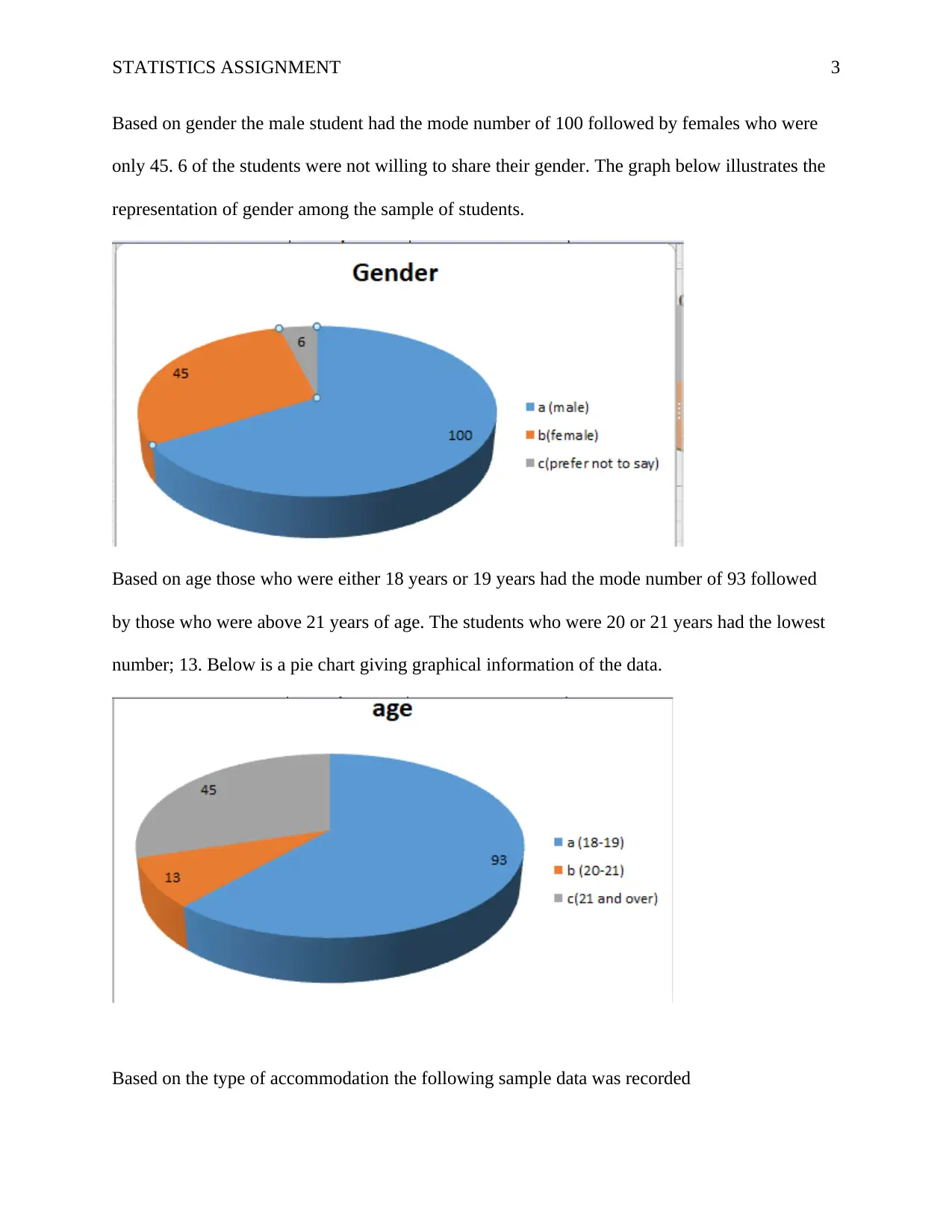
Based on gender the male student had the mode number of 100 followed by females who were
only 45. 6 of the students were not willing to share their gender. The graph below illustrates the
representation of gender among the sample of students.
Based on age those who were either 18 years or 19 years had the mode number of 93 followed
by those who were above 21 years of age. The students who were 20 or 21 years had the lowest
number; 13. Below is a pie chart giving graphical information of the data.
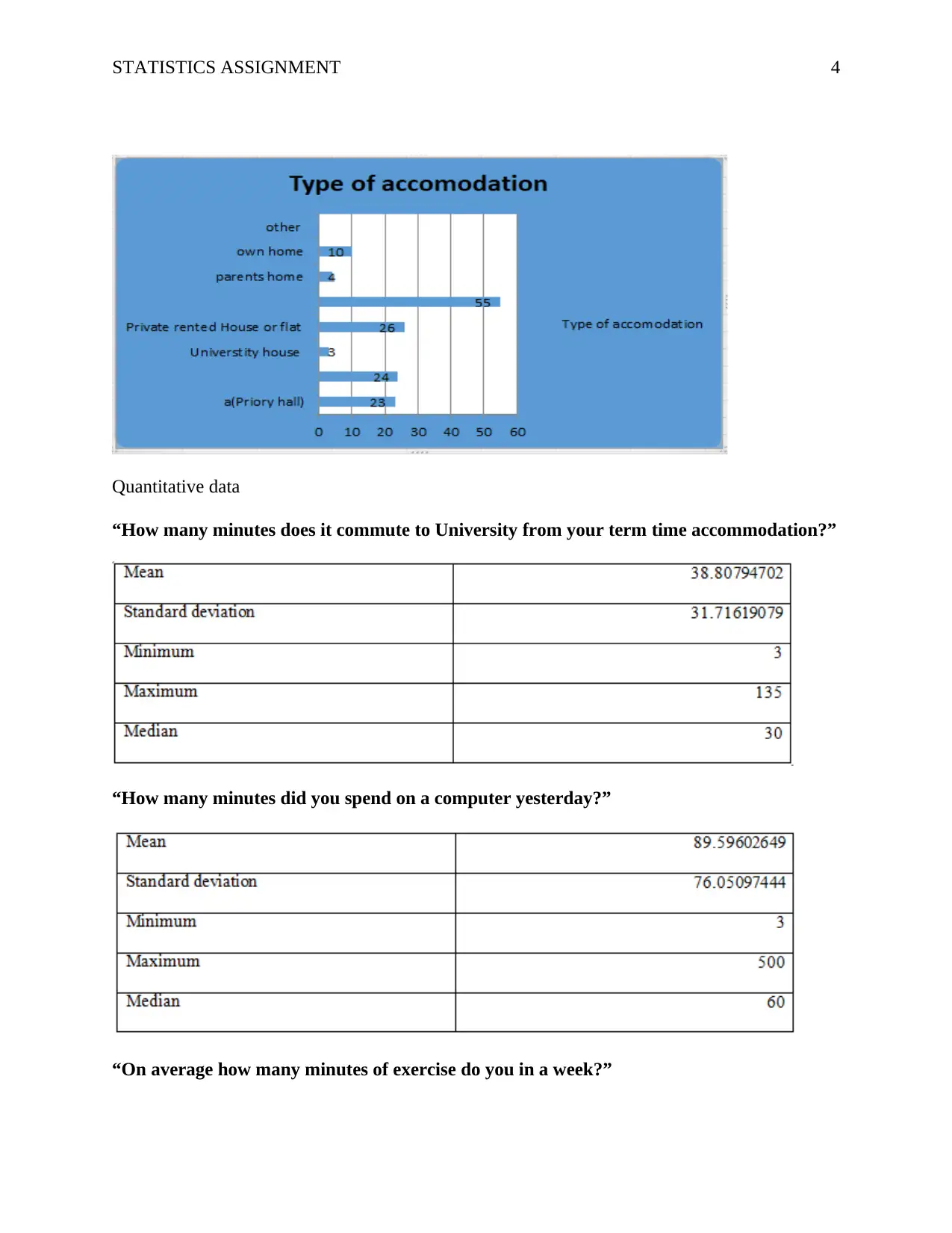
Based on the type of accommodation the following sample data was recorded

STATISTICS ASSIGNMENT 4
Quantitative data
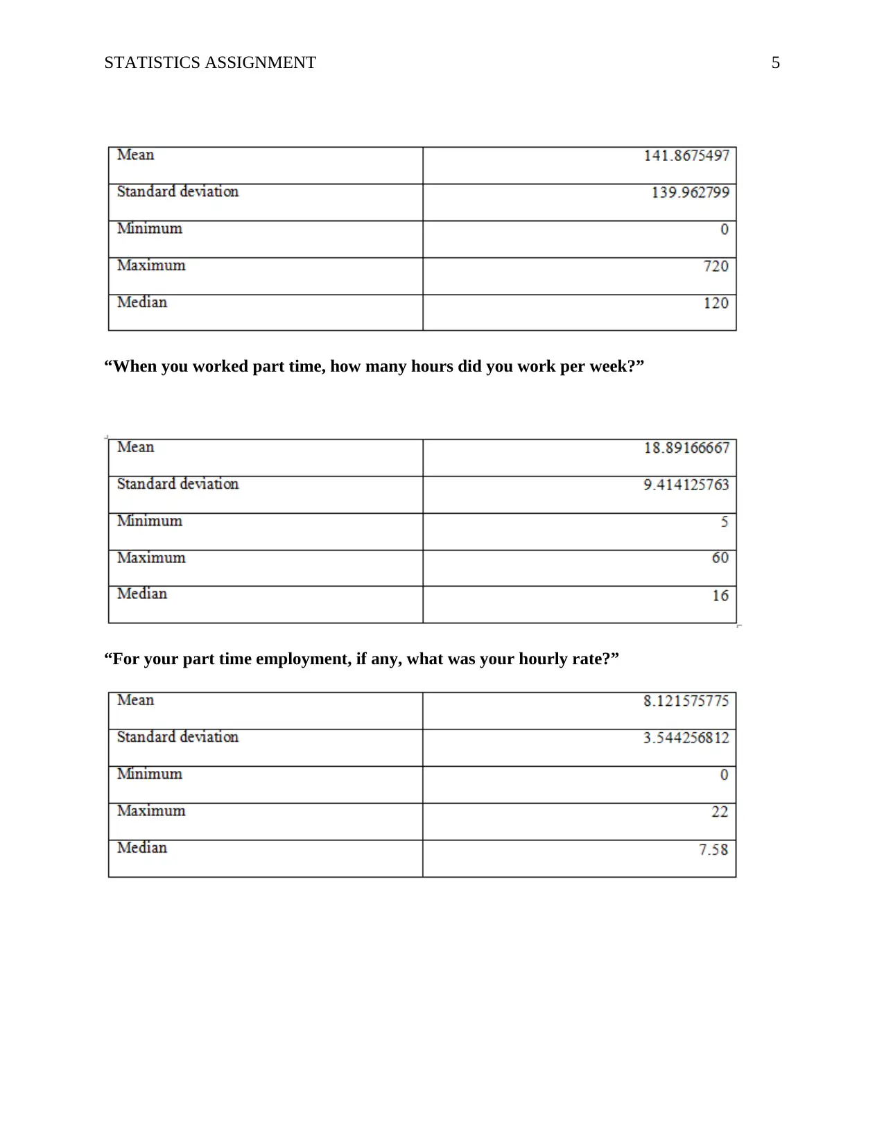
“How many minutes does it commute to University from your term time accommodation?”
“How many minutes did you spend on a computer yesterday?”
“On average how many minutes of exercise do you in a week?”

STATISTICS ASSIGNMENT 5
“When you worked part time, how many hours did you work per week?”
“For your part time employment, if any, what was your hourly rate?”

STATISTICS ASSIGNMENT 6
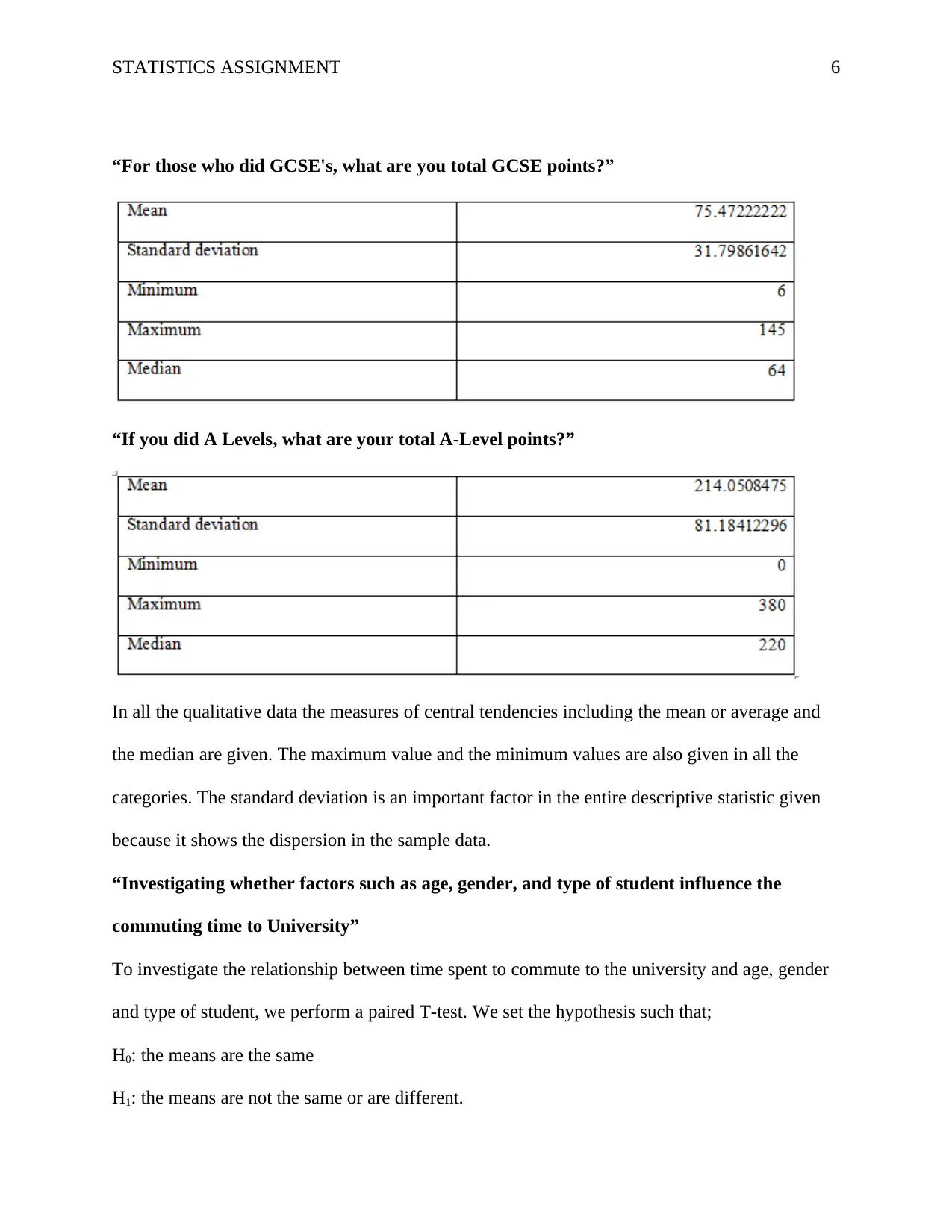
“For those who did GCSE's, what are you total GCSE points?”
“If you did A Levels, what are your total A-Level points?”
In all the qualitative data the measures of central tendencies including the mean or average and
the median are given. The maximum value and the minimum values are also given in all the
categories. The standard deviation is an important factor in the entire descriptive statistic given
because it shows the dispersion in the sample data.
“Investigating whether factors such as age, gender, and type of student influence the
commuting time to University”
To investigate the relationship between time spent to commute to the university and age, gender
and type of student, we perform a paired T-test. We set the hypothesis such that;
H0: the means are the same
H1: the means are not the same or are different.

STATISTICS ASSIGNMENT 7
We reject the null hypothesis if our test statistic t is less than the p= 0.05, a two tailed test (Kim,
2015).
a. Our t = 0.000923, we fail to reject H0 hence the means are the same, we conclude that
gender does not have an effect on the time spent to commute to the university.
b. Our t = 0.971913, we reject the null hypothesis and conclude that there is a relationship
between the type of the student and the time used to commute to the university.
c. Our t = 0.102882, we reject the null hypothesis and conclude that there is no relationship
between the age of the student and the time used to commute to the university from the
term residence.
Conclusion
In summary, the data presents a lot of information regarding the students. Some of the
data is qualitative while others are quantitative. Various descriptive statistics of the data
especially those relating to measure of central tendencies and measure of dispersion are given in
the table (Bickel & Lehmann, 2012). In the second part we compare the effect of various
independent variables such as gender, age, and student type on the time taken for students to
commute. The t-test is utilized to measure the relationships between the three independent
variables (age, student type and gender) on the independent variable which is time taken to
commute from place of accommodation to the university. All the three independent variables do
not affect time of commuting.

STATISTICS ASSIGNMENT 8
Task 2
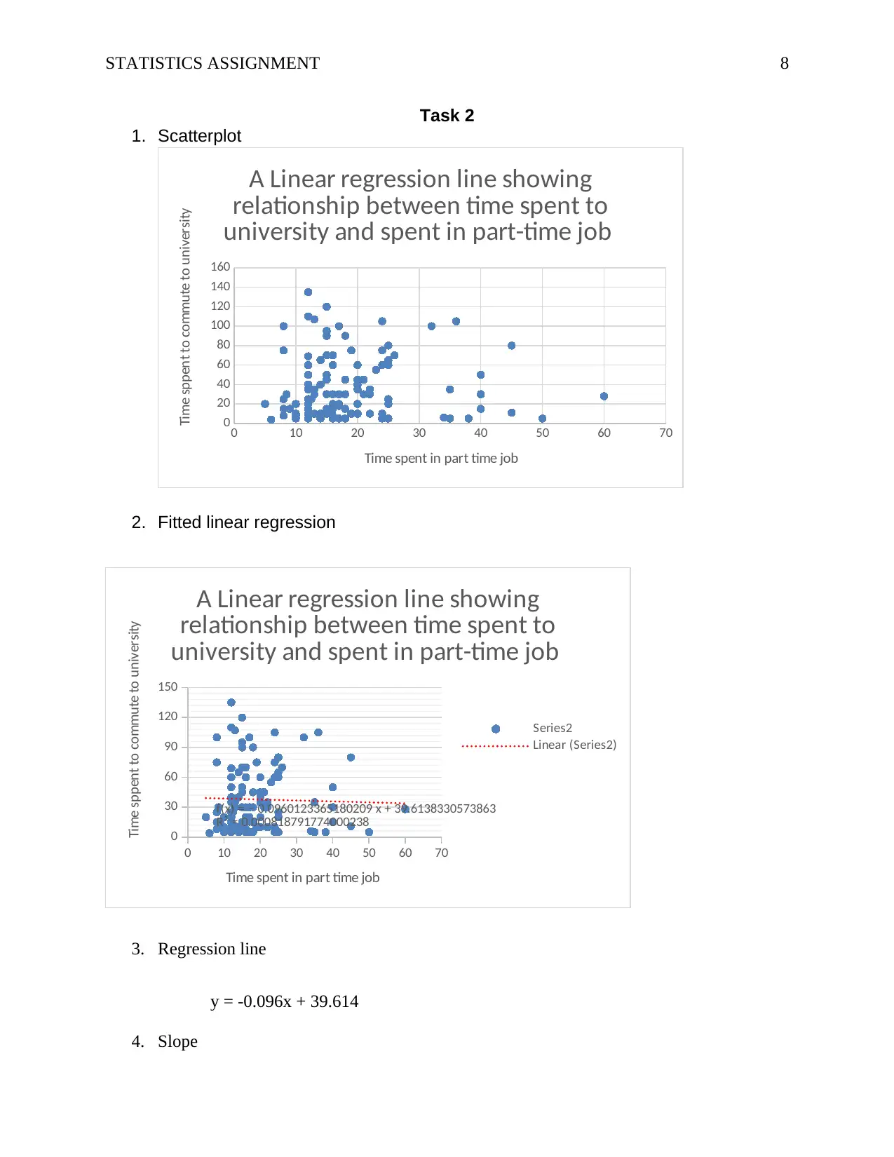
1. Scatterplot
0 10 20 30 40 50 60 70
0
20
40
60
80
100
120
140
160
A Linear regression line showing
relationship between time spent to
university and spent in part-time job
Time spent in part time job
Time sppent to commute to university
2. Fitted linear regression
0 10 20 30 40 50 60 70
0
30
60
90
120
150
f(x) = − 0.0960123365180209 x + 39.6138330573863
R² = 0.000818791774000238
A Linear regression line showing
relationship between time spent to
university and spent in part-time job
Series2
Linear (Series2)
Time spent in part time job
Time sppent to commute to university
3. Regression line
y = -0.096x + 39.614
4. Slope

STATISTICS ASSIGNMENT 9
Slope = -0.09601
The slope shows that an increase in the number of hours spent at the part time job will
result in a decrease in time spent to commute to the university 0.1 minute.
5. Intercept
Intercept = 39.61383
The intercept shows that even if the student did go to the part time job, it would still take
39.61 minutes to commute to the university.
6. R-squared
R-squared = 0.0008
It shows the amount of explained variance, the variance that can be explained by the
independent variable.
7. Prediction
The values are predicted using the regression equation
a. 15 minutes
Y = = -0.096(15) + 39.614
= 38.17 minutes
b. 20 minutes
Y = -0.096(20) + 39.614
= 37.69 minutes
8. Statistically significant test
The test was done using the t-Test for independence.
Null: the means of the two are the same.

STATISTICS ASSIGNMENT 10
Alternative: the means are different (Montgomery, Peck, & Vining,. 2012).
t = 8.41526E-09
Since t <0.05, the two tailed test, we fail to reject the null hypothesis hence there is no
significant result to our mode (Seber & Lee, 2012).
Task 3
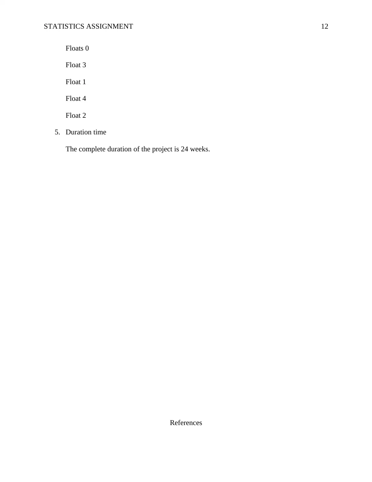
1. Network diagram

STATISTICS ASSIGNMENT 11
2. Preceding diagram
3. Critical path
This is the path which has a float of zero, A – B - K
4. Float associated with each activity
A DC
G
K
B
E F
IH J
0 1
A
0 1
4 8
D
7 1
2
1 4
C
4 7
1 3
G
1 5
2
3
2
9
K
2 2
8 1
0
E
1 1
1
0
1
4
F
1 1
4 8
I
5 1
2
3 4
H
5 5
8 1
2
J
1 1
1 1
0
B
1 1
1
1 3
2
4 2
41 4
4 1
9
2 1 4
9
3 4 2 4 1
4

STATISTICS ASSIGNMENT 12
Floats 0
Float 3
Float 1
Float 4
Float 2
5. Duration time
The complete duration of the project is 24 weeks.
References

STATISTICS ASSIGNMENT 13
Bickel, P. J., & Lehmann, E. L. (2012). Descriptive statistics for nonparametric models I.
Introduction. In Selected Works of EL Lehmann (pp. 465-471). Springer, Boston, MA.
Kim, T. K. (2015). T test as a parametric statistic. Korean journal of anesthesiology, 68(6), 540.
Montgomery, D. C., Peck, E. A., & Vining, G. G. (2012). Introduction to linear regression
analysis (Vol. 821). John Wiley & Sons.
Seber, G. A., & Lee, A. J. (2012). Linear regression analysis (Vol. 329). John Wiley & Sons.