HI6007 Group Assignment: Statistical Data Analysis for Business

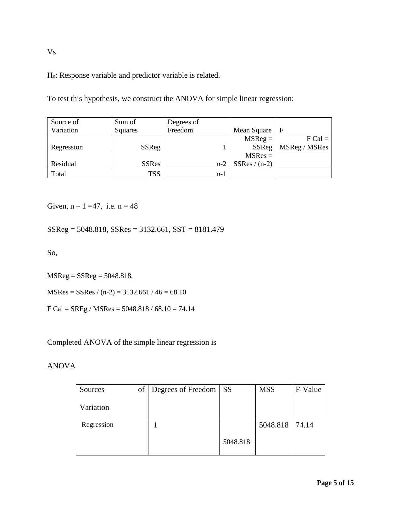
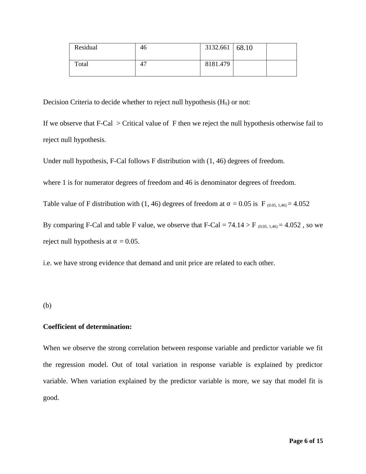
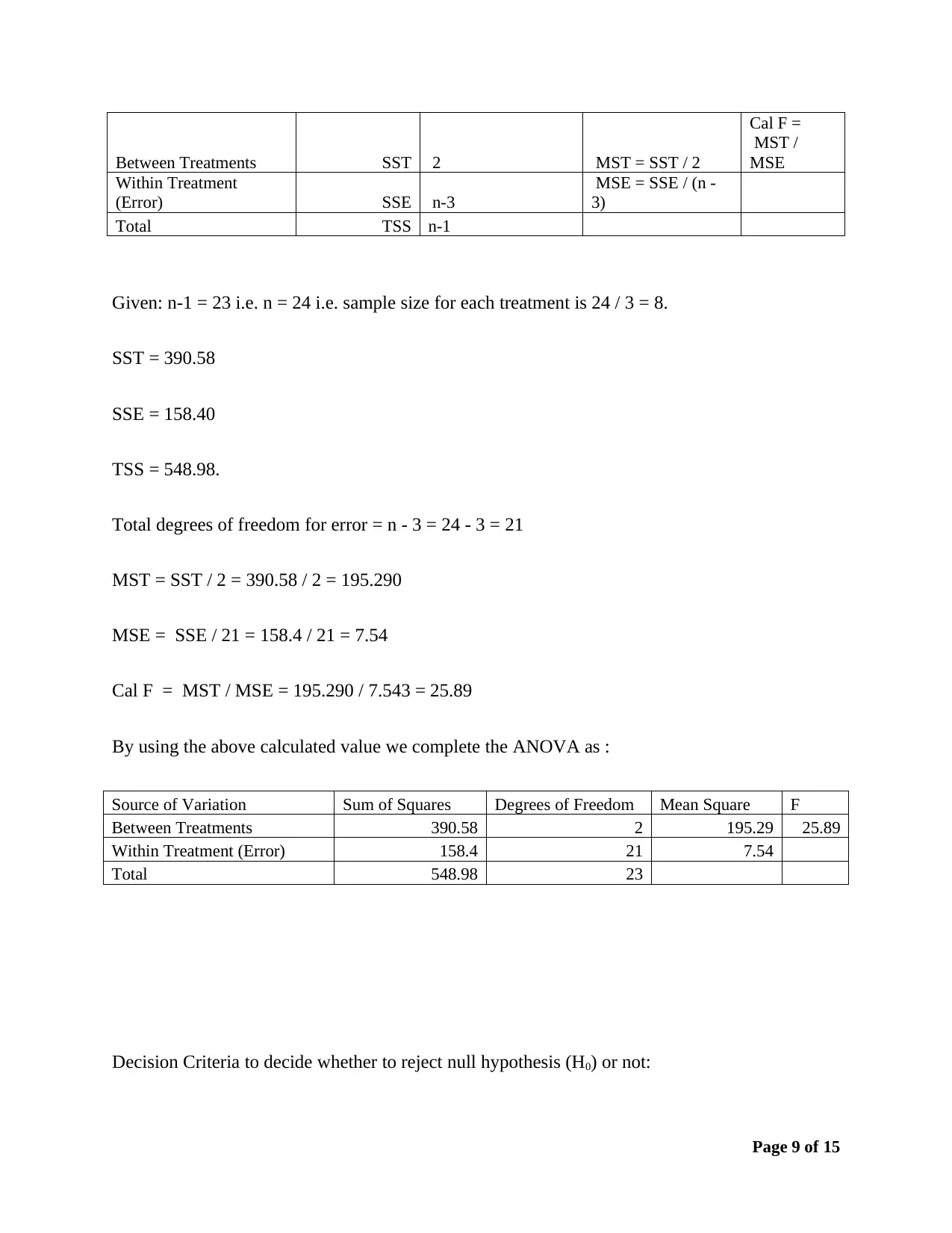
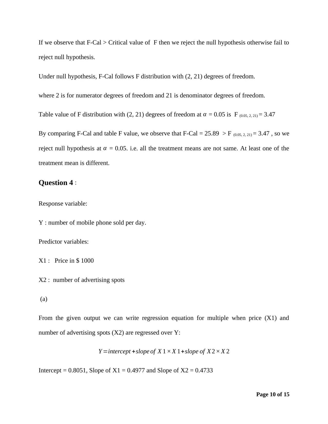
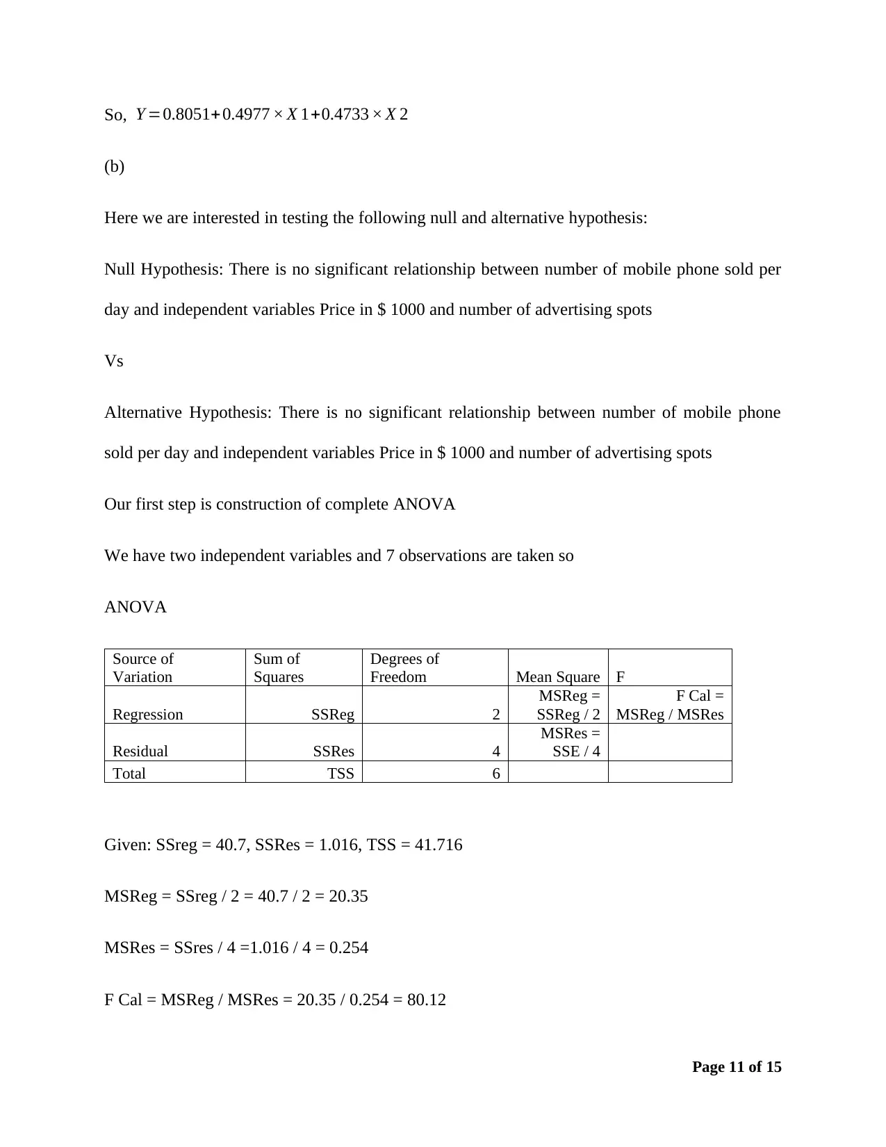
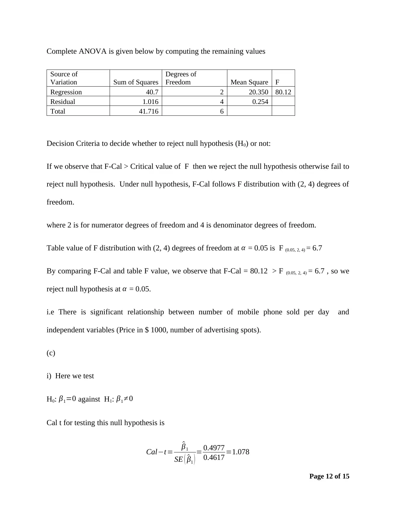
This assignment solution provides a detailed analysis of business data using statistical techniques. It includes the construction of frequency distributions (frequency, relative frequency, and percent frequency) and a histogram to analyze furniture order data. The solution also covers simple linear re...Read More

Solution of the Assignment
Question 1:
Here X : Furniture order (in nearest $)
Min. Obs. = Min { X1, X2, …, X50} ¿ 123
Max. Obs. = Max { X1, X2, …, X50} ¿ 490
So, Range = Max. Obs. – Min. Obs. = 490 -123 = 367
As class width is 50,
Number of classes = (Range) / (class width) = 367 / 50 = 7.340
So we did 7.37 ≈ 8 classes.
We did the classes such that first class include min. obs. and last class include max. obs.
We construct the 8 classes as follows:
120–170 170-220 220-270
270-
320 320-370 370-420 420-470 470-520
Frequency distribution:
Frequency of particular data point means the number of times that data points occurs in the
dataset.
Frequency of the class is the number of data points in that class. Following table shows the
frequency distribution of dataset given for above mentioned classes:
Page 1 of 15

Classes Frequency
120-170 8
170-220 15
220-270 12
270-320 4
320-370 5
370-420 2
420-470 2
470-520 2
Total 50
Relative Frequency distribution:
Relative frequency = Class Frequency / Total number of observations
Classes Relative Frequency
120-
170 0.16
170-
220 0.30
220-
270 0.24
270-
320 0.08
320-
370 0.10
370-
420 0.04
420-
470 0.04
470-
520 0.04
Total 1.00
Page 2 of 15

Percent Frequency distribution:
Percent frequency = Relative frequency × 100
Classes Percent Frequency
120-170 16
170-220 30
220-270 24
270-320 8
320-370 10
370-420 4
420-470 4
470-520 4
Total 100
(b)
Page 3 of 15

Figure : Percent Frequency Histogram
We can observe that positive skewness in the data from percent frequency histogram.
(c)
Mean
Mean is always good measure of location. For our data, Mean = 251.46
Question 2:
Simple linear regression: Where we have only one predictor variable. Here the Response variable
is Demand and Predictor (independent) variable is unit price. We denote,
Y: Demand & X: Unit Price
(a)
H0: Response variable and predictor variable is not related.
Page 4 of 15

Vs
H0: Response variable and predictor variable is related.
To test this hypothesis, we construct the ANOVA for simple linear regression:
Source of
Variation
Sum of
Squares
Degrees of
Freedom Mean Square F
Regression SSReg 1
MSReg =
SSReg
F Cal =
MSReg / MSRes
Residual SSRes n-2
MSRes =
SSRes / (n-2)
Total TSS n-1
Given, n – 1 =47, i.e. n = 48
SSReg = 5048.818, SSRes = 3132.661, SST = 8181.479
So,
MSReg = SSReg = 5048.818,
MSRes = SSRes / (n-2) = 3132.661 / 46 = 68.10
F Cal = SREg / MSRes = 5048.818 / 68.10 = 74.14
Completed ANOVA of the simple linear regression is
ANOVA
Sources of
Variation
Degrees of Freedom SS MSS F-Value
Regression 1
5048.818
5048.818 74.14
Page 5 of 15

Residual 46 3132.661 68.10
Total 47 8181.479
Decision Criteria to decide whether to reject null hypothesis (H0) or not:
If we observe that F-Cal > Critical value of F then we reject the null hypothesis otherwise fail to
reject null hypothesis.
Under null hypothesis, F-Cal follows F distribution with (1, 46) degrees of freedom.
where 1 is for numerator degrees of freedom and 46 is denominator degrees of freedom.
Table value of F distribution with (1, 46) degrees of freedom at α = 0.05 is F (0.05, 1,46) = 4.052
By comparing F-Cal and table F value, we observe that F-Cal = 74.14 > F (0.05, 1,46) = 4.052 , so we
reject null hypothesis at α = 0.05.
i.e. we have strong evidence that demand and unit price are related to each other.
(b)
Coefficient of determination:
When we observe the strong correlation between response variable and predictor variable we fit
the regression model. Out of total variation in response variable is explained by predictor
variable. When variation explained by the predictor variable is more, we say that model fit is
good.
Page 6 of 15

Coefficient of determination is the proportion of variation explained by the predictor variable
from the total variation. Coefficient of determination is denoted by R2 and given by
Coefficient of determination = SSReg / TSS
where TSS is total sum of square.
Alternatively it is defined as
Coefficient of determination = 1 - SSRes / TSS
Coefficient of determination (R2) = 1 - 3132.661 / 8181.479 = 0.6171
It means that 61.71% variation in response (Demand) is explained by the predictor variable (unit
price).
(c)
Correlation coefficient:
Correlation coefficient is denoted by r. We know that Coefficient of determination i.e. R2 is the
square of correlation coefficient (r). So we calculate the r by square root of R2. From slope of X,
we can say that there is negative correlation between X and Y.
So,
r = - √ R2
r = - √0.617103 = - 0.7856
Relationship between demand and unit price:
Page 7 of 15

We observed that correlation coefficient is -0.7856, suggest that demand and unit price is
strongly negatively related with each other.
We can say that when unit price decreases the demand increases and when unit price increases
demand will decreases.
Question 3:
Here we have three treatments.
Let μ1 is the population mean of first treatment, μ2 is the population mean of second treatment
And μ3 is the population mean of third treatment.
Our null and alternative hypothesis are
H0: μ1 = μ2 = μ3
Vs
H1: At least one of μi different. i = 1, 2, 3
For testing the above null hypothesis vs alternative hypothesis, we need to have complete the
ANOVA.
We have 3 treatments and total observations are n then for testing the above hypothesis,
ANOVA is.
Source of Variation
Sum of
Squares Degrees of Freedom Mean Square F
Page 8 of 15

Between Treatments SST 2 MST = SST / 2
Cal F =
MST /
MSE
Within Treatment
(Error) SSE n-3
MSE = SSE / (n -
3)
Total TSS n-1
Given: n-1 = 23 i.e. n = 24 i.e. sample size for each treatment is 24 / 3 = 8.
SST = 390.58
SSE = 158.40
TSS = 548.98.
Total degrees of freedom for error = n - 3 = 24 - 3 = 21
MST = SST / 2 = 390.58 / 2 = 195.290
MSE = SSE / 21 = 158.4 / 21 = 7.54
Cal F = MST / MSE = 195.290 / 7.543 = 25.89
By using the above calculated value we complete the ANOVA as :
Source of Variation Sum of Squares Degrees of Freedom Mean Square F
Between Treatments 390.58 2 195.29 25.89
Within Treatment (Error) 158.4 21 7.54
Total 548.98 23
Decision Criteria to decide whether to reject null hypothesis (H0) or not:
Page 9 of 15

If we observe that F-Cal > Critical value of F then we reject the null hypothesis otherwise fail to
reject null hypothesis.
Under null hypothesis, F-Cal follows F distribution with (2, 21) degrees of freedom.
where 2 is for numerator degrees of freedom and 21 is denominator degrees of freedom.
Table value of F distribution with (2, 21) degrees of freedom at α = 0.05 is F (0.05, 2, 21) = 3.47
By comparing F-Cal and table F value, we observe that F-Cal = 25.89 > F (0.05, 2, 21) = 3.47 , so we
reject null hypothesis at α = 0.05. i.e. all the treatment means are not same. At least one of the
treatment mean is different.
Question 4 :
Response variable:
Y : number of mobile phone sold per day.
Predictor variables:
X1 : Price in $ 1000
X2 : number of advertising spots
(a)
From the given output we can write regression equation for multiple when price (X1) and
number of advertising spots (X2) are regressed over Y:
Y =intercept +slope of X 1 × X 1+slope of X 2 × X 2
Intercept = 0.8051, Slope of X1 = 0.4977 and Slope of X2 = 0.4733
Page 10 of 15

So, Y =0.8051+0.4977 × X 1+0.4733 × X 2
(b)
Here we are interested in testing the following null and alternative hypothesis:
Null Hypothesis: There is no significant relationship between number of mobile phone sold per
day and independent variables Price in $ 1000 and number of advertising spots
Vs
Alternative Hypothesis: There is no significant relationship between number of mobile phone
sold per day and independent variables Price in $ 1000 and number of advertising spots
Our first step is construction of complete ANOVA
We have two independent variables and 7 observations are taken so
ANOVA
Source of
Variation
Sum of
Squares
Degrees of
Freedom Mean Square F
Regression SSReg 2
MSReg =
SSReg / 2
F Cal =
MSReg / MSRes
Residual SSRes 4
MSRes =
SSE / 4
Total TSS 6
Given: SSreg = 40.7, SSRes = 1.016, TSS = 41.716
MSReg = SSreg / 2 = 40.7 / 2 = 20.35
MSRes = SSres / 4 =1.016 / 4 = 0.254
F Cal = MSReg / MSRes = 20.35 / 0.254 = 80.12
Page 11 of 15

Complete ANOVA is given below by computing the remaining values
Source of
Variation Sum of Squares
Degrees of
Freedom Mean Square F
Regression 40.7 2 20.350 80.12
Residual 1.016 4 0.254
Total 41.716 6
Decision Criteria to decide whether to reject null hypothesis (H0) or not:
If we observe that F-Cal > Critical value of F then we reject the null hypothesis otherwise fail to
reject null hypothesis. Under null hypothesis, F-Cal follows F distribution with (2, 4) degrees of
freedom.
where 2 is for numerator degrees of freedom and 4 is denominator degrees of freedom.
Table value of F distribution with (2, 4) degrees of freedom at α = 0.05 is F (0.05, 2, 4) = 6.7
By comparing F-Cal and table F value, we observe that F-Cal = 80.12 > F (0.05, 2, 4) = 6.7 , so we
reject null hypothesis at α = 0.05.
i.e There is significant relationship between number of mobile phone sold per day and
independent variables (Price in $ 1000, number of advertising spots).
(c)
i) Here we test
H0: β1=0 against H1: β1 ≠ 0
Cal t for testing this null hypothesis is
Cal−t = ^β1
SE ( ^β1 ) = 0.4977
0.4617 =1.078
Page 12 of 15

Under Null hypothesi, Cal-t follows t distribution with 4 degrees of freedom.
Critical values of t4 at α = 0.05 is
Critical t value = 2.78
Decision criteria:
Reject H0 if |Cal−t |>Critical t Value
Now |1.078| < 2.78 means we fail to reject H0.
ii) Here we test H0: β2=0 vs H1: β2 ≠ 0
Cal-t for testing this hypothesis is
Cal−t= ^β2
SE ( ^β2 ) = 0.4733
0.0387 =12.22997
Under Null hypothesi, Cal-t follows t distribution with 4 degrees of freedom.
Critical values of t4 at α = 0.05 is
Critical t value = 2.78
Decision criteria:
Reject H0 if |Cal−t |>Critical t Value
So |12.22997| > 2.78
So we reject Null hypothesis.
(d)
Interpretation of Slope of X2:
Page 13 of 15

If price is fixed (i.e. X1 is fixed), then each change in one unit in number of advertising spot
(X2), there is 0.4733 numbers of mobile phone sold per day (Y).
(e)
Given: X1 = 20 and X2 = 10
Then
Y= 0.8051 + 0.4977 × X1 + 0.4733 × X2=0.8051 + 0.4977 × 20 + 0.4733 × 10 = 15.492 ≈ 15
15 (approximately) mobile phones expected to sell in a particular day if company charges $
20000 and used 10 advertising spots.
References
i) Bickel, P.J. and Doksum, K.A., 2015. Mathematical statistics: basic ideas and selected
topics, volume I (Vol. 117). CRC Press.
ii) Box, G.E., Hunter, J.S. and Hunter, W.G., 2005. Statistics for experimenters: design,
innovation, and discovery (Vol. 2). New York: Wiley-Interscience.
iii) Chatterjee, S. and Hadi, A.S., 2015. Regression analysis by example. John Wiley & Sons.
iv) DeGroot, M.H. and Schervish, M.J., 2012. Probability and statistics. Pearson Education.
v) Draper, N.R. and Smith, H., 2014. Applied regression analysis(Vol. 326). John Wiley &
Sons.
vi) Hogg, R.V. and Craig, A.T., 1995. Introduction to mathematical statistics.(5""
edition) (pp. 269-278). Upper Saddle River, New Jersey: Prentice Hall.
vii) Montgomery, D.C., 2017. Design and analysis of experiments. John wiley & sons.
Page 14 of 15

viii) Moyé, L. A., Chan, W., & Kapadia, A. S. (2017). Mathematical statistics with
applications. CRC Press.
ix) Ross, S.M., 2014. Introduction to probability and statistics for engineers and scientists.
Academic Press.
x) Ryan, T.P., 2008. Modern regression methods (Vol. 655). John Wiley & Sons.
Page 15 of 15