Statistics for Business and Finance - Desklib Online Library

This document provides statistical analysis on household expenditures on alcohol, meals, fuel, and phone. It also includes a frequency distribution of expenses for utilities, probability calculations, and a contingency table between gender and level of education. The document is relevant for courses on statistics, business, and finance.

Running head: STATISTICS FOR BUSINESS AND FINANCE
Statistics for Business and Finance
Name of Student
Name of University
Author Note

1STATISTICS FOR BUSINESS AND FINANCE
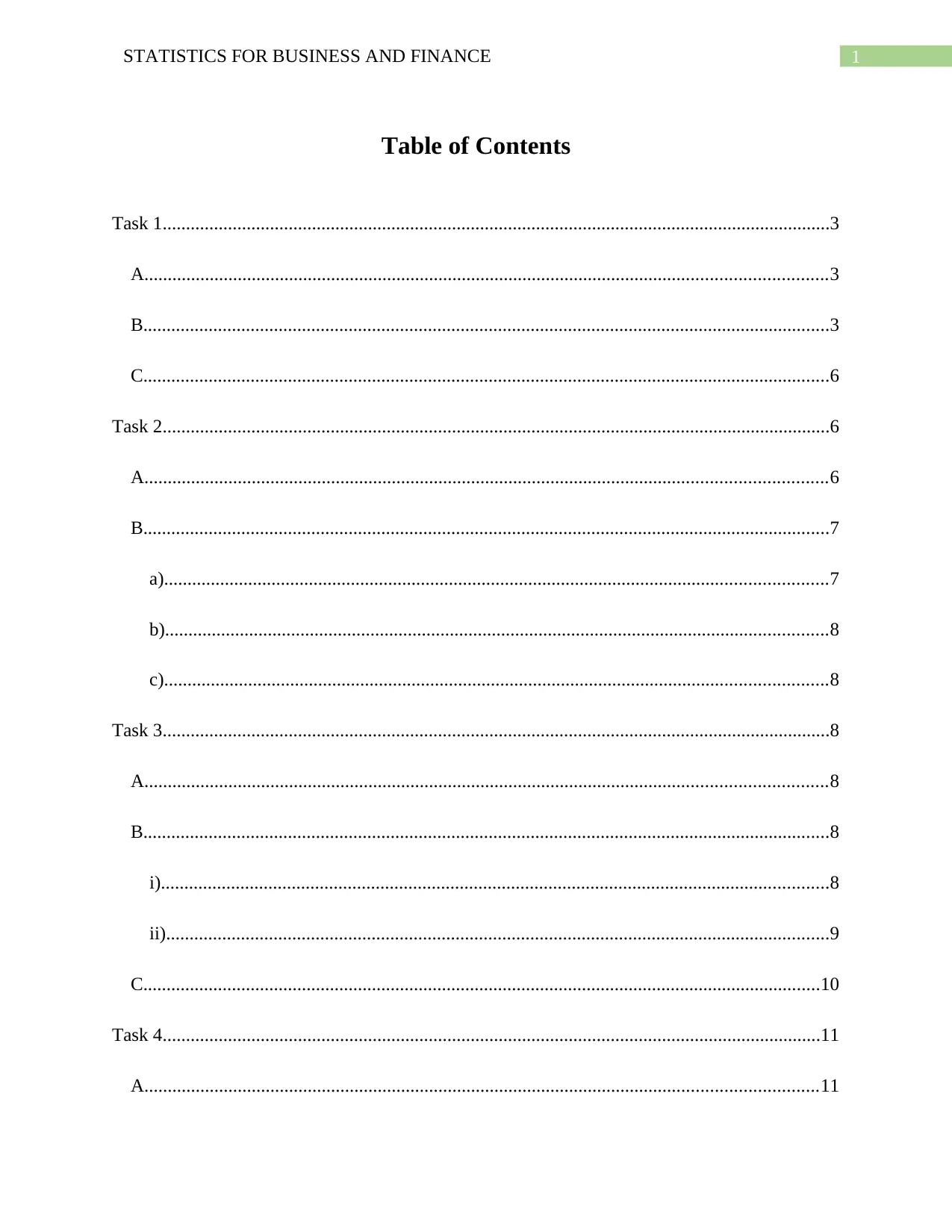
Table of Contents
Task 1...............................................................................................................................................3
A..................................................................................................................................................3
B...................................................................................................................................................3
C...................................................................................................................................................6
Task 2...............................................................................................................................................6
A..................................................................................................................................................6
B...................................................................................................................................................7
a)..............................................................................................................................................7
b)..............................................................................................................................................8
c)..............................................................................................................................................8
Task 3...............................................................................................................................................8
A..................................................................................................................................................8
B...................................................................................................................................................8
i)...............................................................................................................................................8
ii)..............................................................................................................................................9
C.................................................................................................................................................10
Task 4.............................................................................................................................................11
A................................................................................................................................................11

2STATISTICS FOR BUSINESS AND FINANCE
B.................................................................................................................................................11
C.................................................................................................................................................11
D................................................................................................................................................11
E.................................................................................................................................................12

3STATISTICS FOR BUSINESS AND FINANCE
Task 1
A.
A random sample of size 250 was drawn from the given dataset following simple random
sampling procedure. Random numbers, generated using random number generation tool in MS
EXCEL with random seed being 3202(last four digits of student id), were used for the sampling
procedure.
Simple random sampling gives each member of the population an equal chance of being
selected in the sample. Owing to the fact that it is probabilistic in nature it allows for the
mathematical probability of a particular individual or household to be included in the sample. So
the chance of a particular gender or a certain kind of household being the study can be computed.
It is also easy to measure sampling error for this procedure. It is thus suitable for data analysis
and especially inferential data analysis. It is thus free of bias and serves as a representative of the
larger population and would be a good choice in this case.
B.
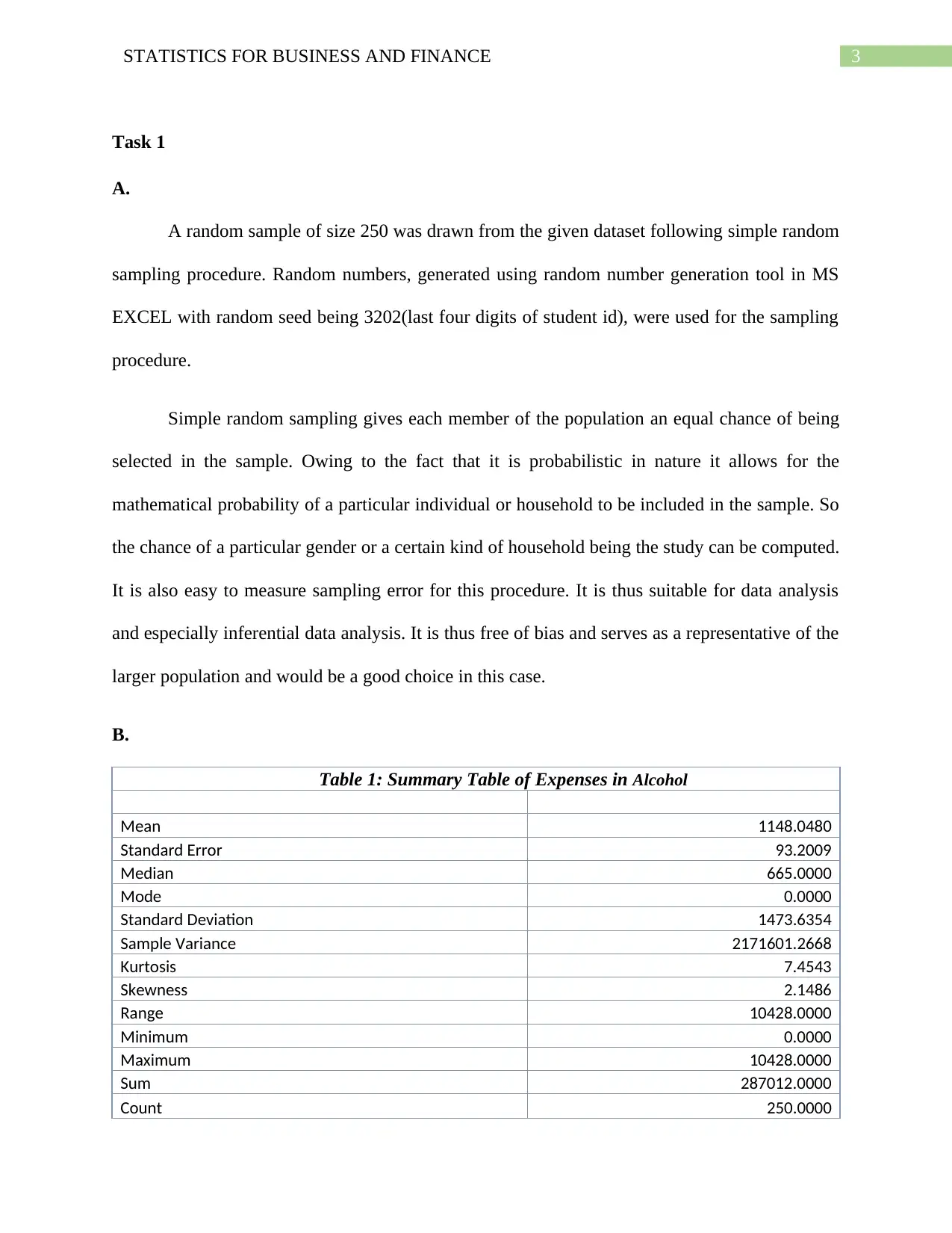
Table 1: Summary Table of Expenses in Alcohol
Mean 1148.0480
Standard Error 93.2009
Median 665.0000
Mode 0.0000
Standard Deviation 1473.6354
Sample Variance 2171601.2668
Kurtosis 7.4543
Skewness 2.1486
Range 10428.0000
Minimum 0.0000
Maximum 10428.0000
Sum 287012.0000
Count 250.0000

4STATISTICS FOR BUSINESS AND FINANCE
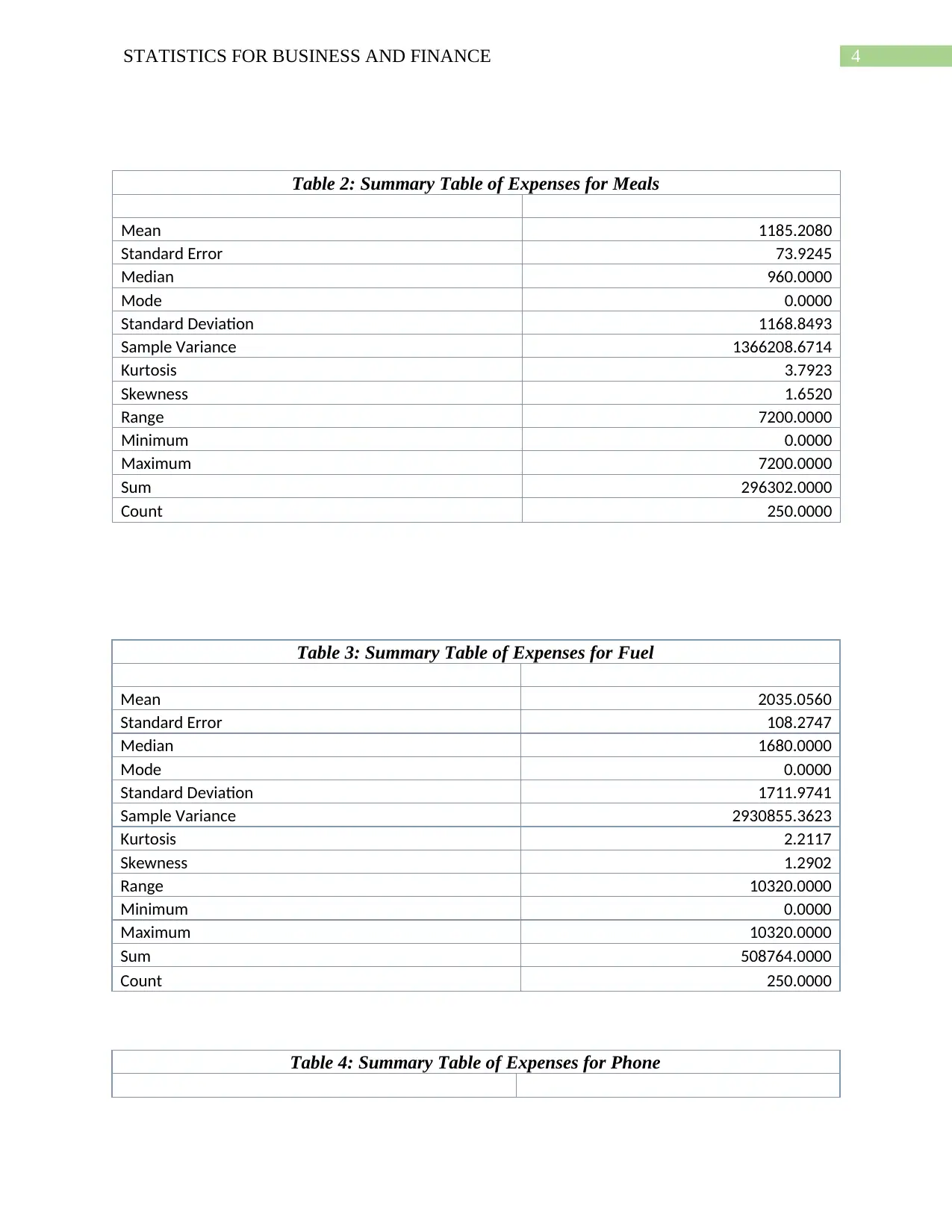
Table 2: Summary Table of Expenses for Meals
Mean 1185.2080
Standard Error 73.9245
Median 960.0000
Mode 0.0000
Standard Deviation 1168.8493
Sample Variance 1366208.6714
Kurtosis 3.7923
Skewness 1.6520
Range 7200.0000
Minimum 0.0000
Maximum 7200.0000
Sum 296302.0000
Count 250.0000
Table 3: Summary Table of Expenses for Fuel
Mean 2035.0560
Standard Error 108.2747
Median 1680.0000
Mode 0.0000
Standard Deviation 1711.9741
Sample Variance 2930855.3623
Kurtosis 2.2117
Skewness 1.2902
Range 10320.0000
Minimum 0.0000
Maximum 10320.0000
Sum 508764.0000
Count 250.0000
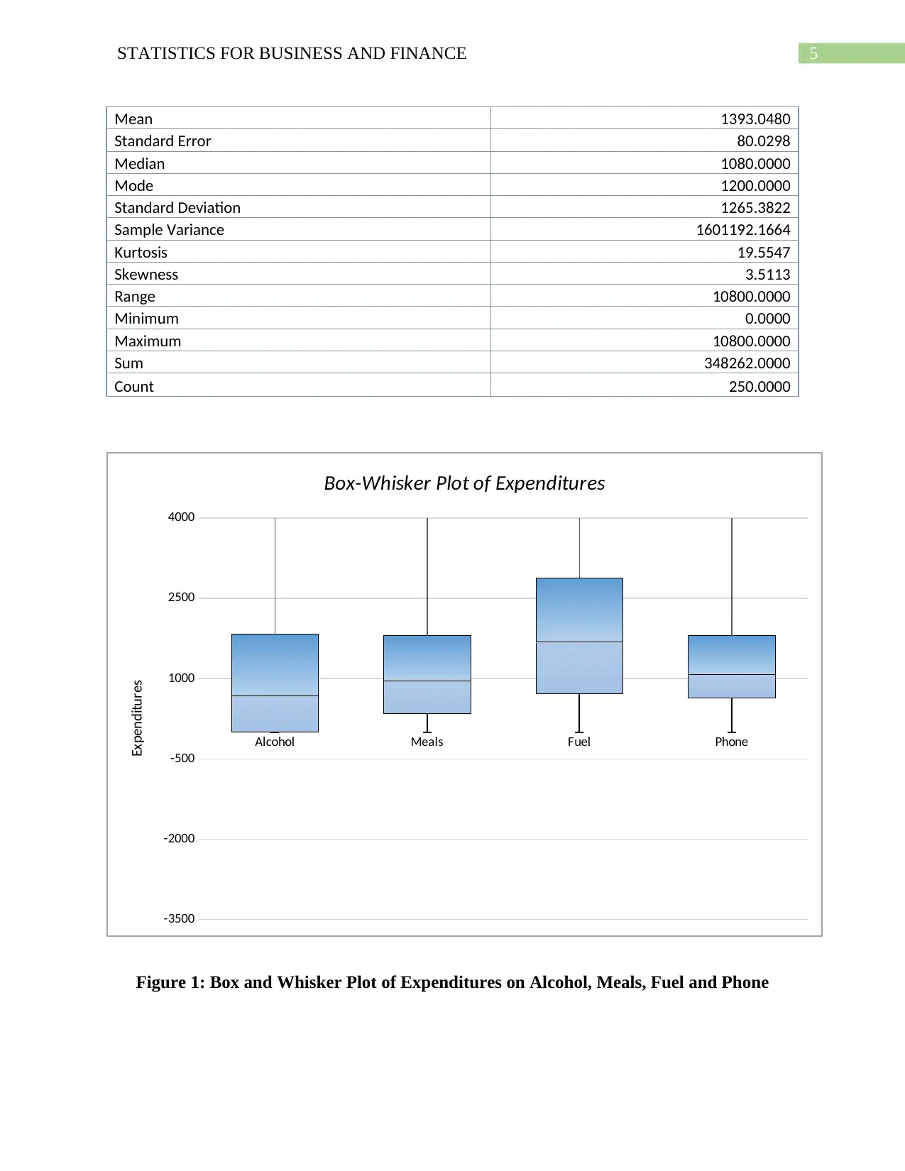
Table 4: Summary Table of Expenses for Phone

5STATISTICS FOR BUSINESS AND FINANCE
Mean 1393.0480
Standard Error 80.0298
Median 1080.0000
Mode 1200.0000
Standard Deviation 1265.3822
Sample Variance 1601192.1664
Kurtosis 19.5547
Skewness 3.5113
Range 10800.0000
Minimum 0.0000
Maximum 10800.0000
Sum 348262.0000
Count 250.0000
Alcohol Meals Fuel Phone
-3500
-2000
-500
1000
2500
4000
Box-Whisker Plot of Expenditures
Expenditures
Figure 1: Box and Whisker Plot of Expenditures on Alcohol, Meals, Fuel and Phone

6STATISTICS FOR BUSINESS AND FINANCE
C.
The mean expenditure on alcohol was found to be 1148.048 with median being 665. It is
thus suggested that the distribution is left skewed. The standard deviation measure has been
observed to be equal to be 1473.63 and so it is understood that the distribution has a large spread.
Comparatively, the mean expenditure was found to be 1185.208 for meals which is lower than
alcohol. The median value of expenditures on meal was however higher than that of alcohol at
960.So even though measure of central tendency, mean suggests that people expend more on
alcohol than meals, median suggests the opposite. It could be argued that perhaps due to outliers,
the situation is distorted for alcohol. The distribution of meals however is also observed to be left
skewed with mean being greater than median. The spread of the distribution of expenditures on
meals is 1168.45 which is less than that for alcohol. The mean for fuel was observed to be
2035.056 which is greater than the mean for both alcohol and meals and the median was found to
be 1680. The central tendency is thus greater than both meals and alcohol. The standard
deviation was observed to be 1711.97 and so spread for fuel is found to be larger than that of
meals and alcohol as well. The average expenditure for phone was observed to be 1393.048 and
its median was found to be 1080, this is lower than fuel expenses and higher than meals and
alcohol.
Task 2
A.
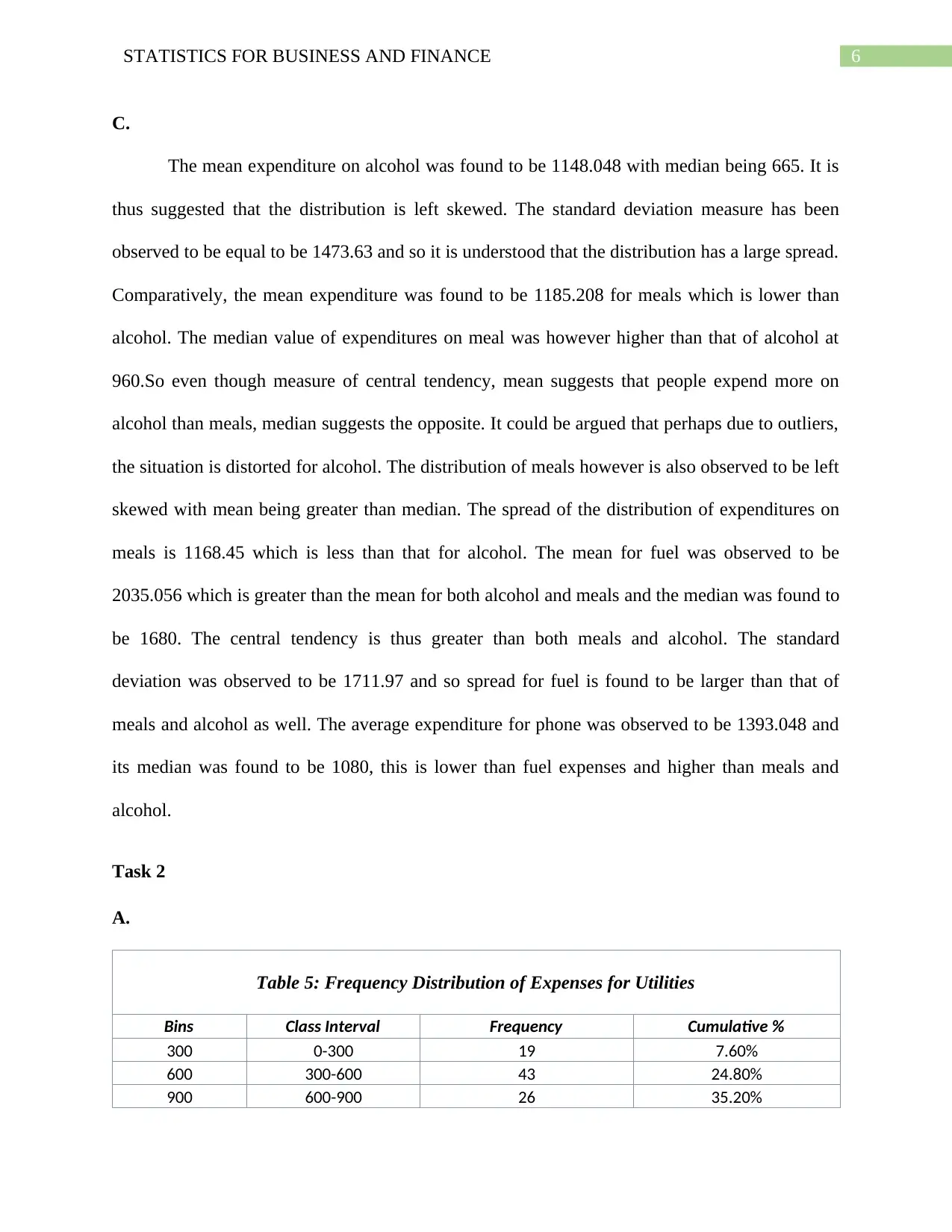
Table 5: Frequency Distribution of Expenses for Utilities
Bins Class Interval Frequency Cumulative %
300 0-300 19 7.60%
600 300-600 43 24.80%
900 600-900 26 35.20%

7STATISTICS FOR BUSINESS AND FINANCE
1200 900-1200 51 55.60%
1500 1200-1500 37 70.40%
1800 1500-1800 24 80.00%
2100 1800-2100 21 88.40%
2400 2100-2400 7 91.20%
2700 2400-2700 6 93.60%
3000 2700-3000 7 96.40%
3300 3000-3300 3 97.60%
3600 3300-3600 0 97.60%
3900 3600-3900 1 98.00%
4100 3900-4100 1 98.40%
4400 4100-4400 0 98.40%
4700 4400-4700 1 98.80%
5000 4700-5000 0 98.80%
5300 5000-5300 0 98.80%
5600 5300-5700 0 98.80%
5900 5700-6100 0 98.80%
6100 6100-6300 0 98.80%
6400 More 3 100.00%
0-300
300-600
600-900
900-1200
1200-1500
1500-1800
1800-2100
2100-2400
2400-2700
2700-3000
3000-3300
3300-3600
3600-3900
3900-4100
4100-4400
4400-4700
4700-5000
5000-5300
5300-5700
5700-6100
6100-6300
More
0
10
20
30
40
50
60
0.00%
20.00%
40.00%
60.00%
80.00%
100.00%
120.00%
Histogram and Ogive of Expense on Utilities
Expense on Utilities
Frequency
% cumulative frequency
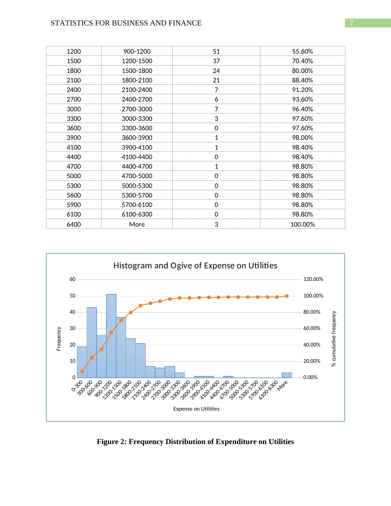
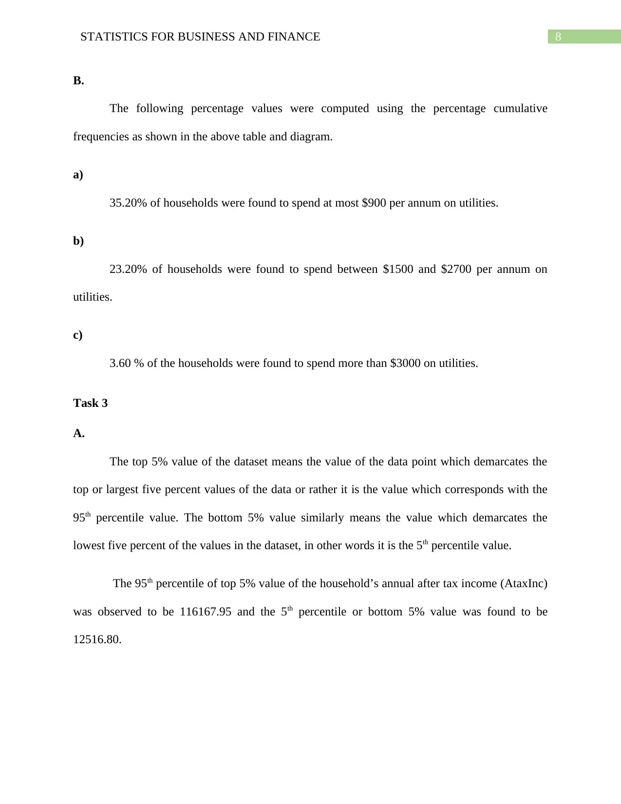
Figure 2: Frequency Distribution of Expenditure on Utilities

8STATISTICS FOR BUSINESS AND FINANCE
B.
The following percentage values were computed using the percentage cumulative
frequencies as shown in the above table and diagram.
a)
35.20% of households were found to spend at most $900 per annum on utilities.
b)
23.20% of households were found to spend between $1500 and $2700 per annum on
utilities.
c)
3.60 % of the households were found to spend more than $3000 on utilities.
Task 3
A.
The top 5% value of the dataset means the value of the data point which demarcates the
top or largest five percent values of the data or rather it is the value which corresponds with the
95th percentile value. The bottom 5% value similarly means the value which demarcates the
lowest five percent of the values in the dataset, in other words it is the 5th percentile value.
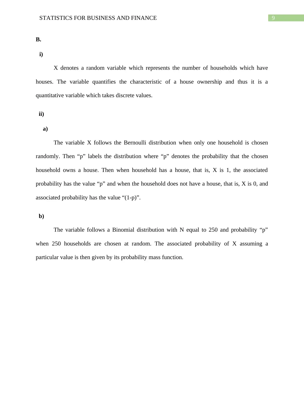
The 95th percentile of top 5% value of the household’s annual after tax income (AtaxInc)
was observed to be 116167.95 and the 5th percentile or bottom 5% value was found to be
12516.80.

9STATISTICS FOR BUSINESS AND FINANCE
B.
i)
X denotes a random variable which represents the number of households which have
houses. The variable quantifies the characteristic of a house ownership and thus it is a
quantitative variable which takes discrete values.
ii)
a)
The variable X follows the Bernoulli distribution when only one household is chosen
randomly. Then “p” labels the distribution where “p” denotes the probability that the chosen
household owns a house. Then when household has a house, that is, X is 1, the associated
probability has the value “p” and when the household does not have a house, that is, X is 0, and
associated probability has the value “(1-p)”.
b)
The variable follows a Binomial distribution with N equal to 250 and probability “p”
when 250 households are chosen at random. The associated probability of X assuming a
particular value is then given by its probability mass function.

10STATISTICS FOR BUSINESS AND FINANCE
C.
8.00000 8.50000 9.00000 9.50000 10.00000 10.50000 11.00000 11.50000
8.00000
9.00000
10.00000
11.00000
12.00000
13.00000
14.00000
Logarithm of total expenditure Vs. logarithm of
annual after tax Income
Natural Log of Annual after Tax Income
Natural log of total expenditure
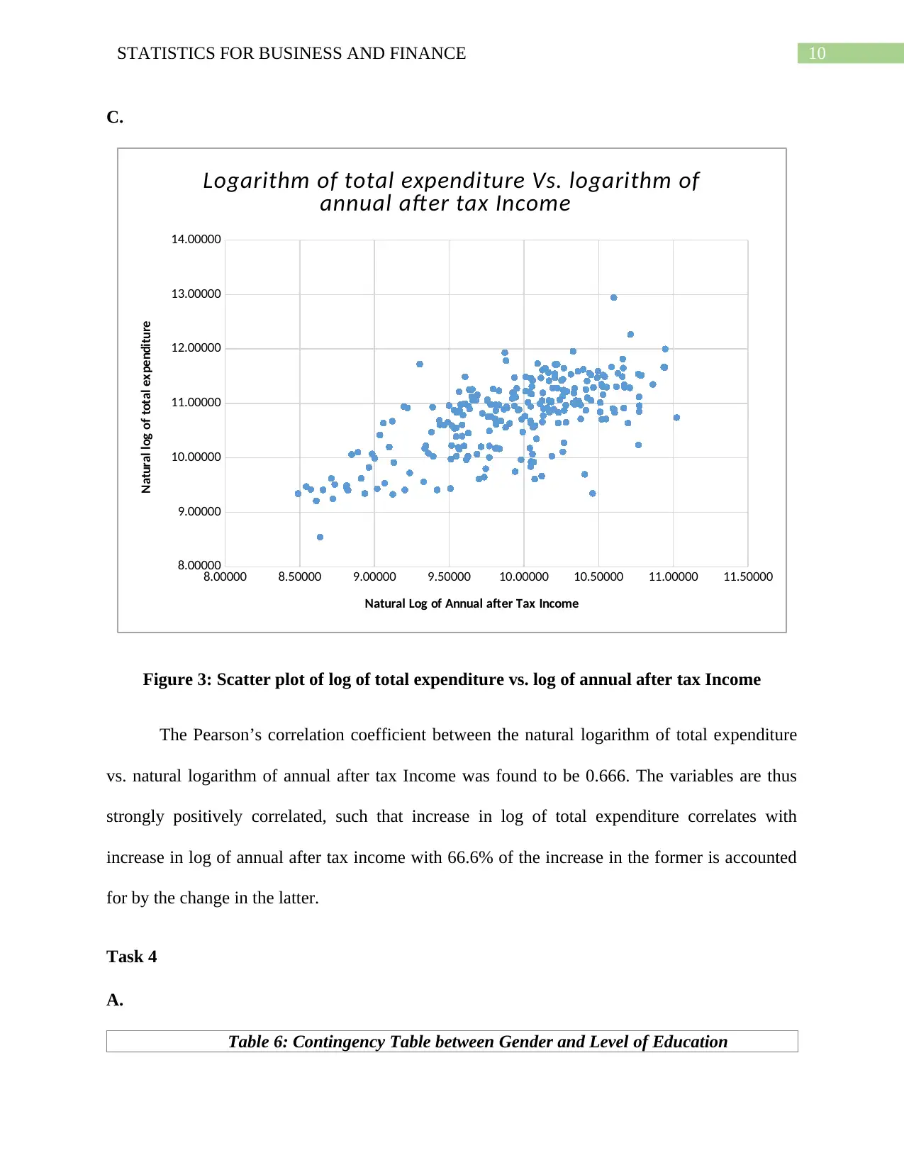
Figure 3: Scatter plot of log of total expenditure vs. log of annual after tax Income
The Pearson’s correlation coefficient between the natural logarithm of total expenditure
vs. natural logarithm of annual after tax Income was found to be 0.666. The variables are thus
strongly positively correlated, such that increase in log of total expenditure correlates with
increase in log of annual after tax income with 66.6% of the increase in the former is accounted
for by the change in the latter.
Task 4
A.
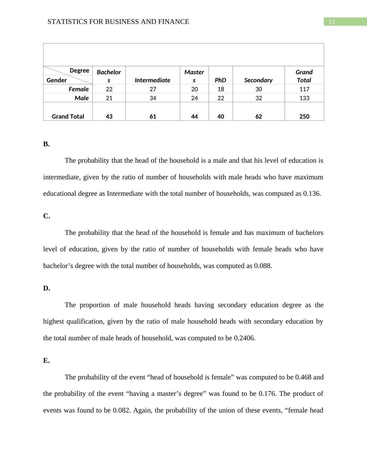
Table 6: Contingency Table between Gender and Level of Education

11STATISTICS FOR BUSINESS AND FINANCE
Degree Bachelor
s Intermediate
Master
s PhD Secondary
Grand
TotalGender
Female 22 27 20 18 30 117
Male 21 34 24 22 32 133
Grand Total 43 61 44 40 62 250
B.
The probability that the head of the household is a male and that his level of education is
intermediate, given by the ratio of number of households with male heads who have maximum
educational degree as Intermediate with the total number of households, was computed as 0.136.
C.
The probability that the head of the household is female and has maximum of bachelors
level of education, given by the ratio of number of households with female heads who have
bachelor’s degree with the total number of households, was computed as 0.088.
D.
The proportion of male household heads having secondary education degree as the
highest qualification, given by the ratio of male household heads with secondary education by
the total number of male heads of household, was computed to be 0.2406.
E.
The probability of the event “head of household is female” was computed to be 0.468 and
the probability of the event “having a master’s degree” was found to be 0.176. The product of
events was found to be 0.082. Again, the probability of the union of these events, “female head

12STATISTICS FOR BUSINESS AND FINANCE
having master’s degree” was found to be 0.082. Therefore the intersection is thus 0.002 which is
approximately 0. The events are thus concluded to be independent.