Statistics. Business intelligence and data visualizatio
VerifiedAdded on 2023/03/30
|16
|2679
|235
AI Summary
1.Conduct data analysis for Web Analytics at Quality Alloys, Inc. Use EXCEL and SPSS to conduct analysis
2) Write a report for Web Analytics at Quality Alloys, Inc. (500-800 words)
Your report should be submitted in two parts. The first part should be an executive summary. It should summarize results and provide recommendations to QA managers as to how they might best market their business with an aim towards improving sales.
The second part of your report should be responses to the questions posed in the Analysis section that follows.
You should do the second part (the quantitative analysis) prior to doing the first part (the executive summary). Be sure to read through the entire case at least once before proceeding.
Make sure you complete all the 10 questions in part 2
Contribute Materials
Your contribution can guide someone’s learning journey. Share your
documents today.

Statistics
Business intelligence and data visualization
Student name:
Tutor name:
1 | P a g e
Business intelligence and data visualization
Student name:
Tutor name:
1 | P a g e
Secure Best Marks with AI Grader
Need help grading? Try our AI Grader for instant feedback on your assignments.

Statistics
Executive summary
This research study was focused on analyzing the information retrieved from QA website and
uses the results for decision making. The results showed that despite having a new website, the
revenue over the period of test remained generally constant. The research recommends to the QA
management to create a platform within the website to allow customers make and possibly pay
for orders. The management should also look for other robust advertising methods to advertise
their products.
2 | P a g e
Statistics
Question 1
Unique visits to the QA website per week
May 25 - May 31
Jun 15 - Jun 21
Jul 6 - Jul 12
Jul 27 - Aug 2
Aug 17 - Aug 23
Sep 7 - Sep 13
Sep 28 - Oct 4
Oct 19 - Oct 25
Nov 9 - Nov 15
Nov 30 - Dec 6
Dec 21 - Dec 27
Jan 11 - Jan 17
Feb 1 - Feb 7
Feb 22 - Feb 28
Mar 15 - Mar 21
Apr 5 - Apr 11
Apr 26 - May 2
May 17 - May 23
Jun 7 - Jun 13
Jun 28 - Jul 4
Jul 19 - Jul 25
Aug 9 - Aug 15
0
500
1,000
1,500
2,000
2,500
3,000
3,500
4,000
Unique Visits to the QA
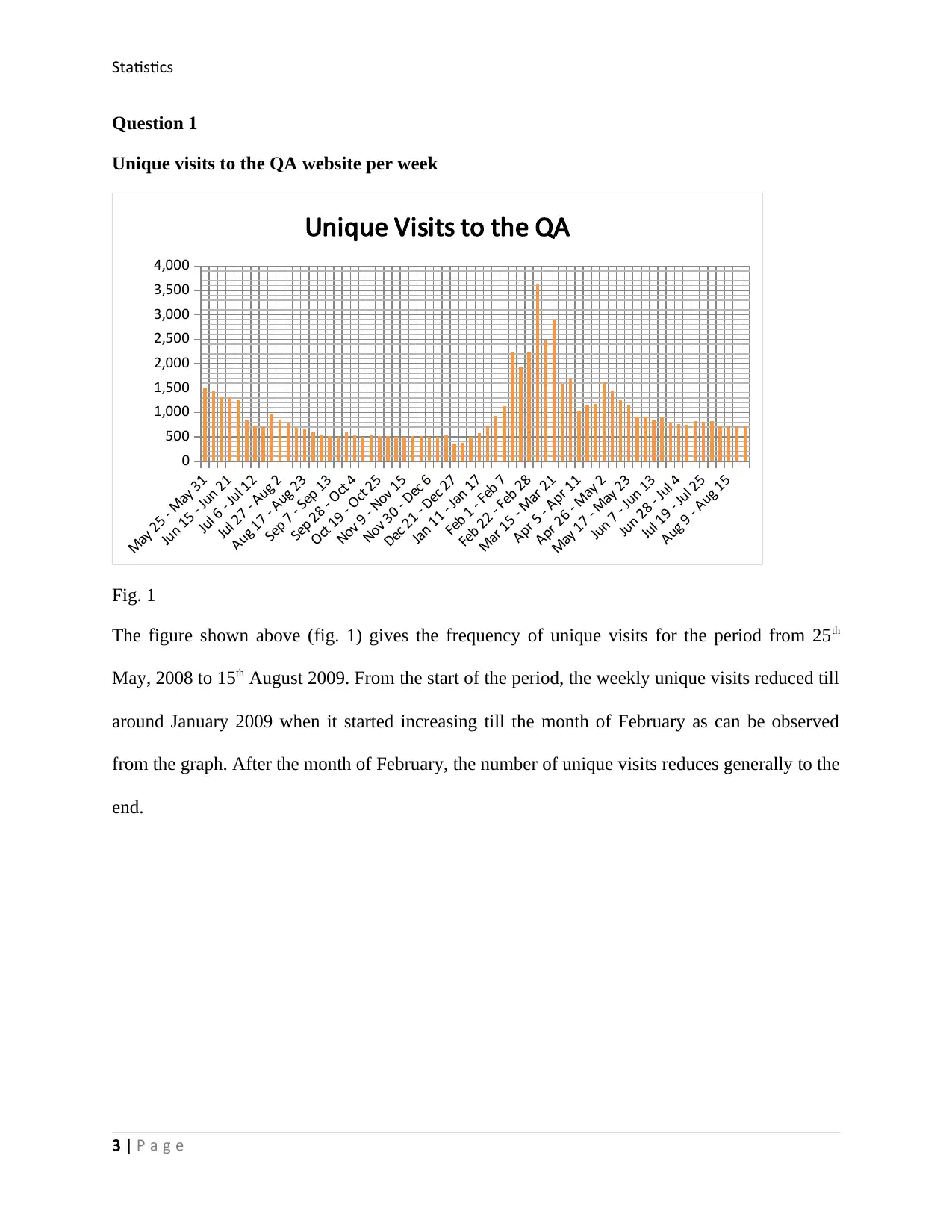
Fig. 1
The figure shown above (fig. 1) gives the frequency of unique visits for the period from 25th
May, 2008 to 15th August 2009. From the start of the period, the weekly unique visits reduced till
around January 2009 when it started increasing till the month of February as can be observed
from the graph. After the month of February, the number of unique visits reduces generally to the
end.
3 | P a g e
Statistics
Distribution of revenue every week
May 25 - May 31
Jun 22 - Jun 28
Jul 20 - Jul 26
Aug 17 - Aug 23
Sep 14 - Sep 20
Oct 12 - Oct 18
Nov 9 - Nov 15
Dec 7 - Dec 13
Jan 4 - Jan 10
Feb 1 - Feb 7
Mar 1 - Mar 7
Mar 29 - Apr 4
Apr 26 - May 2
May 24 - May 30
Jun 21 - Jun 27
Jul 19 - Jul 25
Aug 16 - Aug 22
$0
$100,000
$200,000
$300,000
$400,000
$500,000
$600,000
$700,000
$800,000
$900,000
$1,000,000
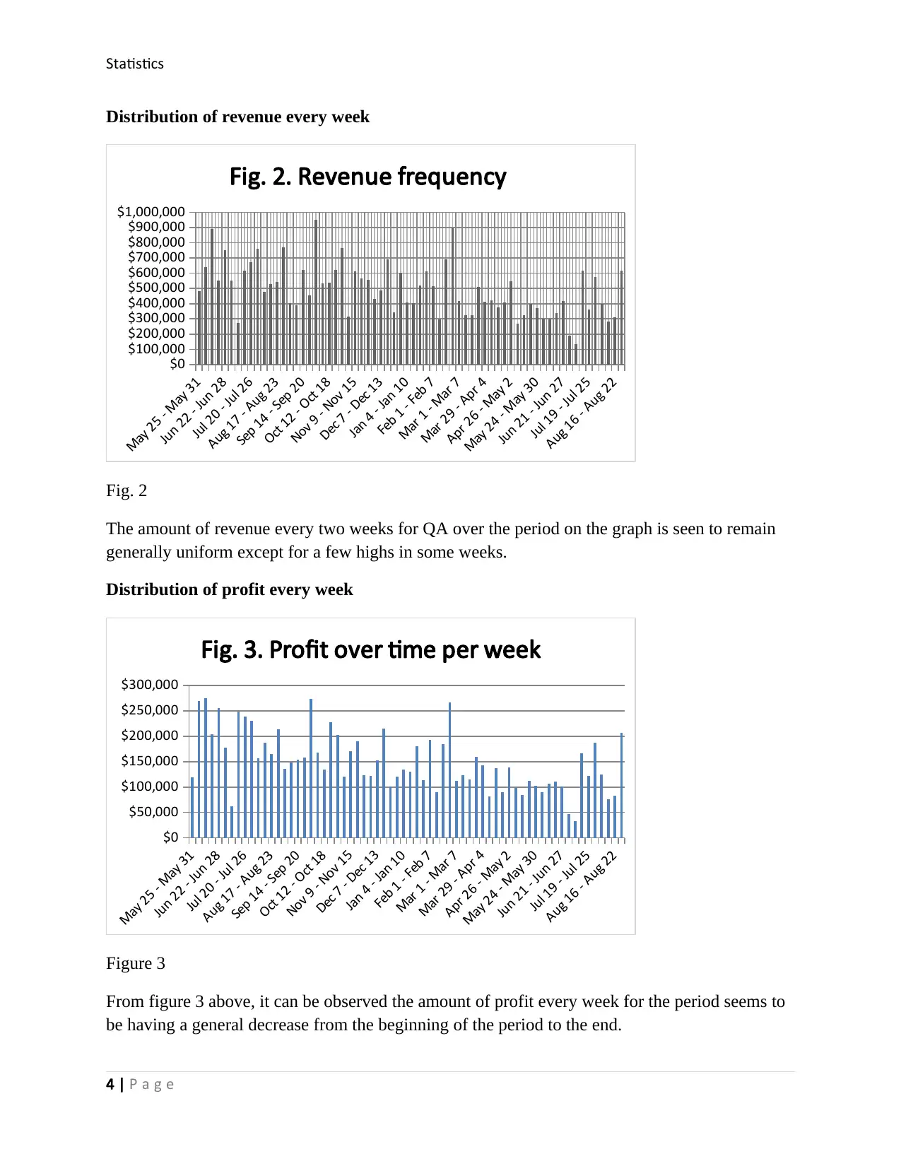
Fig. 2. Revenue frequency
Fig. 2
The amount of revenue every two weeks for QA over the period on the graph is seen to remain
generally uniform except for a few highs in some weeks.
Distribution of profit every week
May 25 - May 31
Jun 22 - Jun 28
Jul 20 - Jul 26
Aug 17 - Aug 23
Sep 14 - Sep 20
Oct 12 - Oct 18
Nov 9 - Nov 15
Dec 7 - Dec 13
Jan 4 - Jan 10
Feb 1 - Feb 7
Mar 1 - Mar 7
Mar 29 - Apr 4
Apr 26 - May 2
May 24 - May 30
Jun 21 - Jun 27
Jul 19 - Jul 25
Aug 16 - Aug 22
$0
$50,000
$100,000
$150,000
$200,000
$250,000
$300,000
Fig. 3. Profit over time per week
Figure 3
From figure 3 above, it can be observed the amount of profit every week for the period seems to
be having a general decrease from the beginning of the period to the end.
4 | P a g e
Secure Best Marks with AI Grader
Need help grading? Try our AI Grader for instant feedback on your assignments.
Statistics
Distribution of pounds sold for the period
May 25 - May 31
Jun 22 - Jun 28
Jul 20 - Jul 26
Aug 17 - Aug 23
Sep 14 - Sep 20
Oct 12 - Oct 18
Nov 9 - Nov 15
Dec 7 - Dec 13
Jan 4 - Jan 10
Feb 1 - Feb 7
Mar 1 - Mar 7
Mar 29 - Apr 4
Apr 26 - May 2
May 24 - May 30
Jun 21 - Jun 27
Jul 19 - Jul 25
Aug 16 - Aug 22
0
5,000
10,000
15,000
20,000
25,000
30,000
35,000
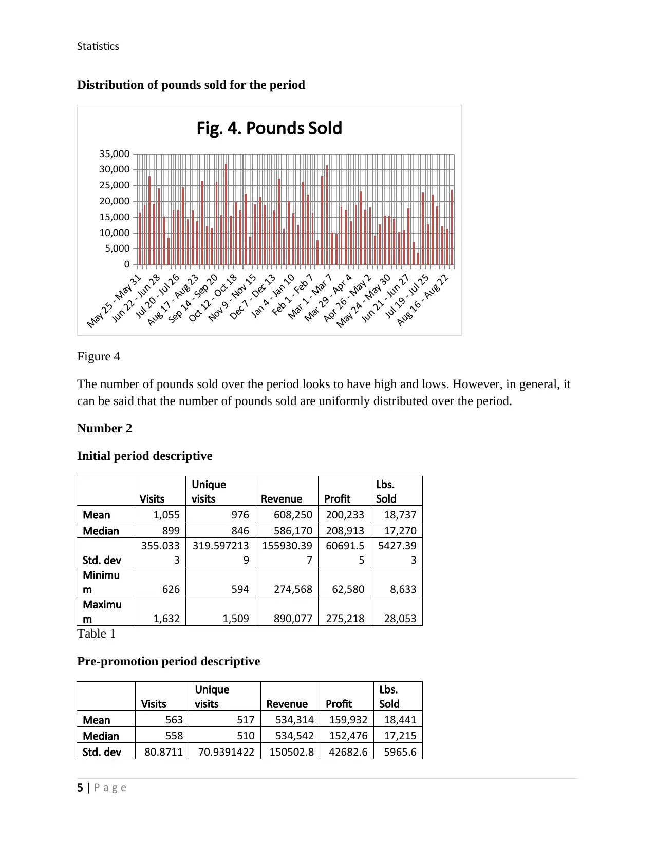
Fig. 4. Pounds Sold
Figure 4
The number of pounds sold over the period looks to have high and lows. However, in general, it
can be said that the number of pounds sold are uniformly distributed over the period.
Number 2
Initial period descriptive
Visits
Unique
visits Revenue Profit
Lbs.
Sold
Mean 1,055 976 608,250 200,233 18,737
Median 899 846 586,170 208,913 17,270
Std. dev
355.033
3
319.597213
9
155930.39
7
60691.5
5
5427.39
3
Minimu
m 626 594 274,568 62,580 8,633
Maximu
m 1,632 1,509 890,077 275,218 28,053
Table 1
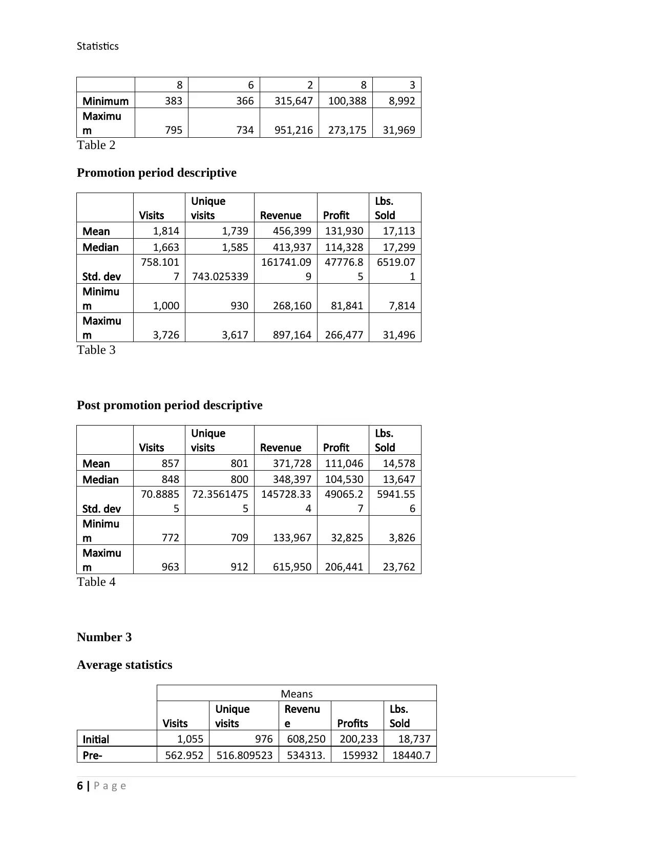
Pre-promotion period descriptive
Visits
Unique
visits Revenue Profit
Lbs.
Sold
Mean 563 517 534,314 159,932 18,441
Median 558 510 534,542 152,476 17,215
Std. dev 80.8711 70.9391422 150502.8 42682.6 5965.6
5 | P a g e
Statistics
8 6 2 8 3
Minimum 383 366 315,647 100,388 8,992
Maximu
m 795 734 951,216 273,175 31,969
Table 2
Promotion period descriptive
Visits
Unique
visits Revenue Profit
Lbs.
Sold
Mean 1,814 1,739 456,399 131,930 17,113
Median 1,663 1,585 413,937 114,328 17,299
Std. dev
758.101
7 743.025339
161741.09
9
47776.8
5
6519.07
1
Minimu
m 1,000 930 268,160 81,841 7,814
Maximu
m 3,726 3,617 897,164 266,477 31,496
Table 3
Post promotion period descriptive
Visits
Unique
visits Revenue Profit
Lbs.
Sold
Mean 857 801 371,728 111,046 14,578
Median 848 800 348,397 104,530 13,647
Std. dev
70.8885
5
72.3561475
5
145728.33
4
49065.2
7
5941.55
6
Minimu
m 772 709 133,967 32,825 3,826
Maximu
m 963 912 615,950 206,441 23,762
Table 4
Number 3
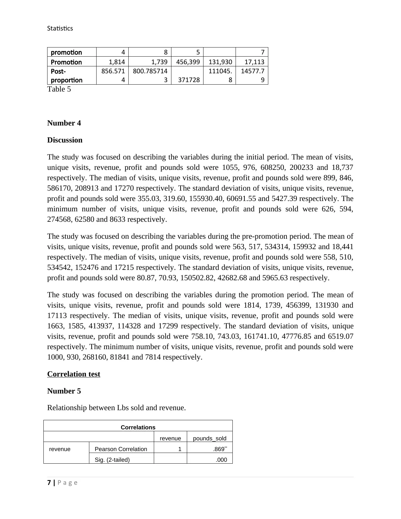
Average statistics
Means
Visits
Unique
visits
Revenu
e Profits
Lbs.
Sold
Initial 1,055 976 608,250 200,233 18,737
Pre- 562.952 516.809523 534313. 159932 18440.7
6 | P a g e
Statistics
promotion 4 8 5 7
Promotion 1,814 1,739 456,399 131,930 17,113
Post-
proportion
856.571
4
800.785714
3 371728
111045.
8
14577.7
9
Table 5
Number 4
Discussion
The study was focused on describing the variables during the initial period. The mean of visits,
unique visits, revenue, profit and pounds sold were 1055, 976, 608250, 200233 and 18,737
respectively. The median of visits, unique visits, revenue, profit and pounds sold were 899, 846,
586170, 208913 and 17270 respectively. The standard deviation of visits, unique visits, revenue,
profit and pounds sold were 355.03, 319.60, 155930.40, 60691.55 and 5427.39 respectively. The
minimum number of visits, unique visits, revenue, profit and pounds sold were 626, 594,
274568, 62580 and 8633 respectively.
The study was focused on describing the variables during the pre-promotion period. The mean of
visits, unique visits, revenue, profit and pounds sold were 563, 517, 534314, 159932 and 18,441
respectively. The median of visits, unique visits, revenue, profit and pounds sold were 558, 510,
534542, 152476 and 17215 respectively. The standard deviation of visits, unique visits, revenue,
profit and pounds sold were 80.87, 70.93, 150502.82, 42682.68 and 5965.63 respectively.
The study was focused on describing the variables during the promotion period. The mean of
visits, unique visits, revenue, profit and pounds sold were 1814, 1739, 456399, 131930 and
17113 respectively. The median of visits, unique visits, revenue, profit and pounds sold were
1663, 1585, 413937, 114328 and 17299 respectively. The standard deviation of visits, unique
visits, revenue, profit and pounds sold were 758.10, 743.03, 161741.10, 47776.85 and 6519.07
respectively. The minimum number of visits, unique visits, revenue, profit and pounds sold were
1000, 930, 268160, 81841 and 7814 respectively.
Correlation test
Number 5
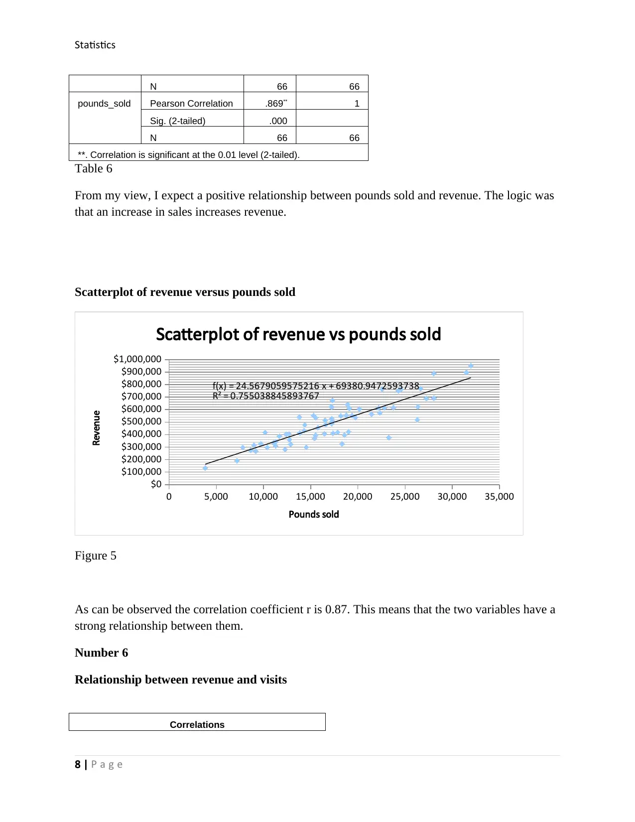
Relationship between Lbs sold and revenue.
Correlations
revenue pounds_sold
revenue Pearson Correlation 1 .869**
Sig. (2-tailed) .000
7 | P a g e
Paraphrase This Document
Need a fresh take? Get an instant paraphrase of this document with our AI Paraphraser
Statistics
N 66 66
pounds_sold Pearson Correlation .869** 1
Sig. (2-tailed) .000
N 66 66
**. Correlation is significant at the 0.01 level (2-tailed).
Table 6
From my view, I expect a positive relationship between pounds sold and revenue. The logic was
that an increase in sales increases revenue.
Scatterplot of revenue versus pounds sold
0 5,000 10,000 15,000 20,000 25,000 30,000 35,000
$0
$100,000
$200,000
$300,000
$400,000
$500,000
$600,000
$700,000
$800,000
$900,000
$1,000,000
f(x) = 24.5679059575216 x + 69380.9472593738
R² = 0.755038845893767
Scatterplot of revenue vs pounds sold
Pounds sold
Revenue
Figure 5
As can be observed the correlation coefficient r is 0.87. This means that the two variables have a
strong relationship between them.
Number 6
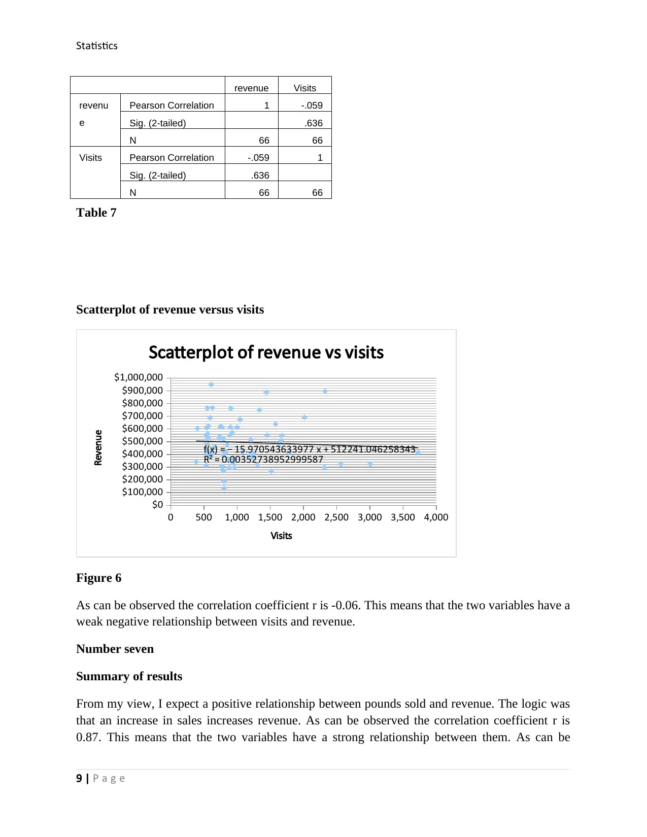
Relationship between revenue and visits
Correlations
8 | P a g e
N 66 66
pounds_sold Pearson Correlation .869** 1
Sig. (2-tailed) .000
N 66 66
**. Correlation is significant at the 0.01 level (2-tailed).
Table 6
From my view, I expect a positive relationship between pounds sold and revenue. The logic was
that an increase in sales increases revenue.
Scatterplot of revenue versus pounds sold
0 5,000 10,000 15,000 20,000 25,000 30,000 35,000
$0
$100,000
$200,000
$300,000
$400,000
$500,000
$600,000
$700,000
$800,000
$900,000
$1,000,000
f(x) = 24.5679059575216 x + 69380.9472593738
R² = 0.755038845893767
Scatterplot of revenue vs pounds sold
Pounds sold
Revenue
Figure 5
As can be observed the correlation coefficient r is 0.87. This means that the two variables have a
strong relationship between them.
Number 6
Relationship between revenue and visits
Correlations
8 | P a g e
Statistics
revenue Visits
revenu
e
Pearson Correlation 1 -.059
Sig. (2-tailed) .636
N 66 66
Visits Pearson Correlation -.059 1
Sig. (2-tailed) .636
N 66 66
Table 7
Scatterplot of revenue versus visits
0 500 1,000 1,500 2,000 2,500 3,000 3,500 4,000
$0
$100,000
$200,000
$300,000
$400,000
$500,000
$600,000
$700,000
$800,000
$900,000
$1,000,000
f(x) = − 15.970543633977 x + 512241.046258343
R² = 0.00352738952999587
Scatterplot of revenue vs visits
Visits
Revenue
Figure 6
As can be observed the correlation coefficient r is -0.06. This means that the two variables have a
weak negative relationship between visits and revenue.
Number seven
Summary of results
From my view, I expect a positive relationship between pounds sold and revenue. The logic was
that an increase in sales increases revenue. As can be observed the correlation coefficient r is
0.87. This means that the two variables have a strong relationship between them. As can be
9 | P a g e
Statistics
observed the correlation coefficient r between revenue and visit is -0.06. This means that the two
variables have a weak negative relationship between visits and revenue.
Number eight
a. Descriptive statistics for pounds sold for the period
Results tableLbs. Sold
Mean 18681.5551
7
Median 17673
Std Dev. 6840.50794
Min. 3826
Max. 44740
Table 8
It can be observed that the mean 18681.55. The median number of pounds sold was 17673 while
the standard deviation was 6840.5.
b. Histogram of pounds sold
Figure 7
10 | P a g e
Secure Best Marks with AI Grader
Need help grading? Try our AI Grader for instant feedback on your assignments.
Statistics
c. The distribution of the number of pounds sold over the period is normally distributed as
can be observed from the shape of the curve.
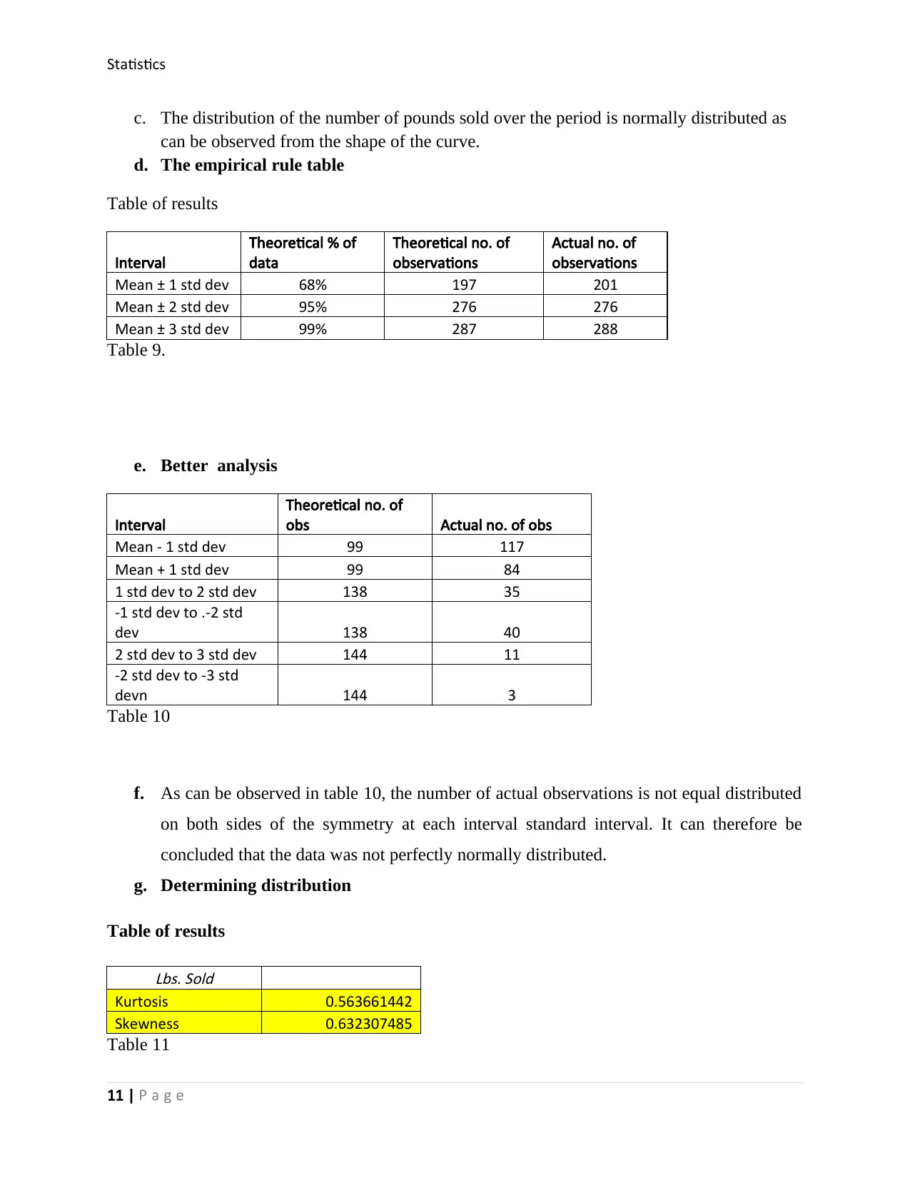
d. The empirical rule table
Table of results
Interval
Theoretical % of
data
Theoretical no. of
observations
Actual no. of
observations
Mean ± 1 std dev 68% 197 201
Mean ± 2 std dev 95% 276 276
Mean ± 3 std dev 99% 287 288
Table 9.
e. Better analysis
Interval
Theoretical no. of
obs Actual no. of obs
Mean - 1 std dev 99 117
Mean + 1 std dev 99 84
1 std dev to 2 std dev 138 35
-1 std dev to .-2 std
dev 138 40
2 std dev to 3 std dev 144 11
-2 std dev to -3 std
devn 144 3
Table 10
f. As can be observed in table 10, the number of actual observations is not equal distributed
on both sides of the symmetry at each interval standard interval. It can therefore be
concluded that the data was not perfectly normally distributed.
g. Determining distribution
Table of resultsLbs. Sold
Kurtosis 0.563661442
Skewness 0.632307485
Table 11
11 | P a g e
Statistics
In this case the skewness value is 0.63 which is close to zero. This means an almost normal
distribution. The kurtosis value of 0.56 also means that the distribution has a low and broad peak.
Number 9
Distribution pounds and visit
The skewness for visits was 2.17 and that of pounds sold was 0.63. It can therefore be concluded
that the distribution of visits was more skewed than pounds sold hence not normally distributed.
Number 10
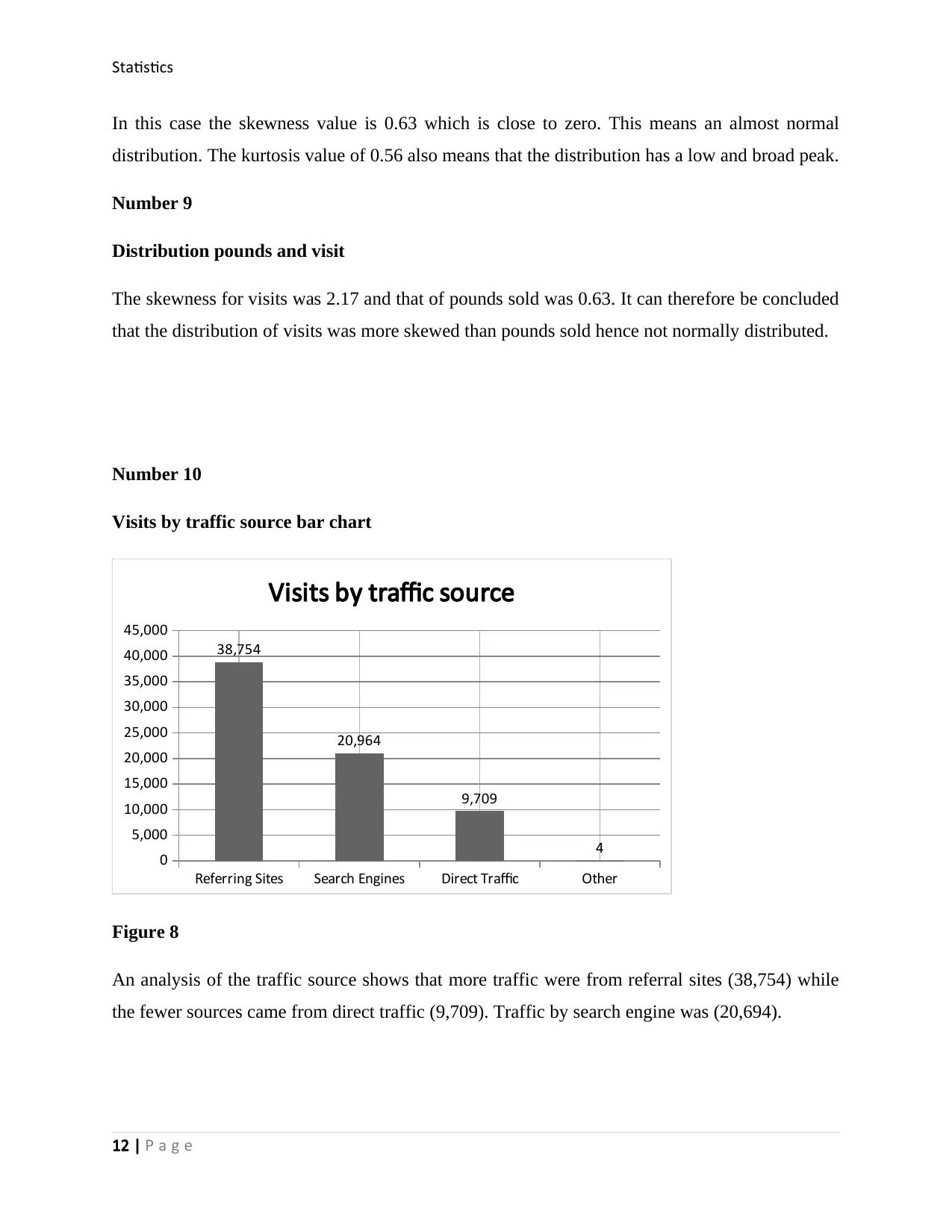
Visits by traffic source bar chart
Referring Sites Search Engines Direct Traffic Other
0
5,000
10,000
15,000
20,000
25,000
30,000
35,000
40,000
45,000
38,754
20,964
9,709
4
Visits by traffic source
Figure 8
An analysis of the traffic source shows that more traffic were from referral sites (38,754) while
the fewer sources came from direct traffic (9,709). Traffic by search engine was (20,694).
12 | P a g e
Statistics
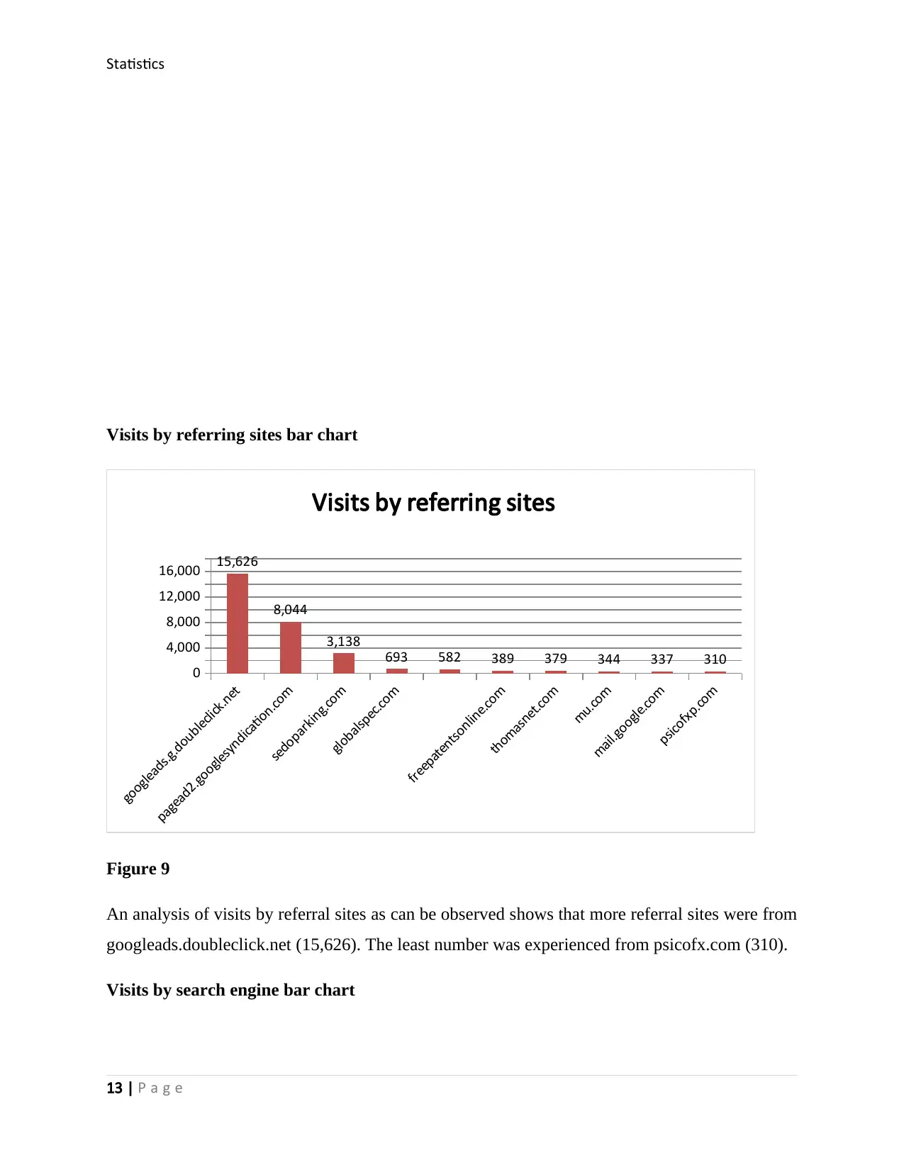
Visits by referring sites bar chart
googleads.g.doubleclick.net
pagead2.googlesyndication.com
sedoparking.com
globalspec.com
freepatentsonline.com
thomasnet.com
mu.com
mail.google.com
psicofxp.com
0
4,000
8,000
12,000
16,000 15,626
8,044
3,138
693 582 389 379 344 337 310
Visits by referring sites
Figure 9
An analysis of visits by referral sites as can be observed shows that more referral sites were from
googleads.doubleclick.net (15,626). The least number was experienced from psicofx.com (310).
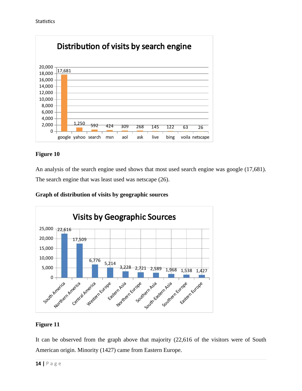
Visits by search engine bar chart
13 | P a g e
Paraphrase This Document
Need a fresh take? Get an instant paraphrase of this document with our AI Paraphraser
Statistics
google yahoo search msn aol ask live bing voila netscape
0
2,000
4,000
6,000
8,000
10,000
12,000
14,000
16,000
18,000
20,000 17,681
1,250 592 424 309 268 145 122 63 26
Distribution of visits by search engine
Figure 10
An analysis of the search engine used shows that most used search engine was google (17,681).
The search engine that was least used was netscape (26).
Graph of distribution of visits by geographic sources
South America
Northern America
Central America
Western Europe
Eastern Asia
Northern Europe
Southern Asia
South-Eastern Asia
Southern Europe
Eastern Europe
0
5,000
10,000
15,000
20,000
25,000 22,616
17,509
6,776 5,214 3,228 2,721 2,589 1,968 1,538 1,427
Visits by Geographic Sources
Figure 11
It can be observed from the graph above that majority (22,616 of the visitors were of South
American origin. Minority (1427) came from Eastern Europe.
14 | P a g e
Statistics
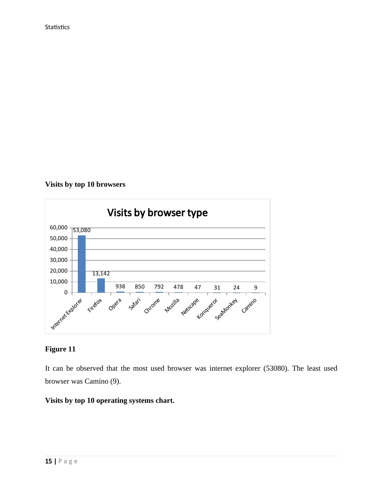
Visits by top 10 browsers
Internet Explorer
Firefox
Opera
Safari
Chrome
Mozilla
Netscape
Konqueror
SeaMonkey
Camino
0
10,000
20,000
30,000
40,000
50,000
60,000 53,080
13,142
938 850 792 478 47 31 24 9
Visits by browser type
Figure 11
It can be observed that the most used browser was internet explorer (53080). The least used
browser was Camino (9).
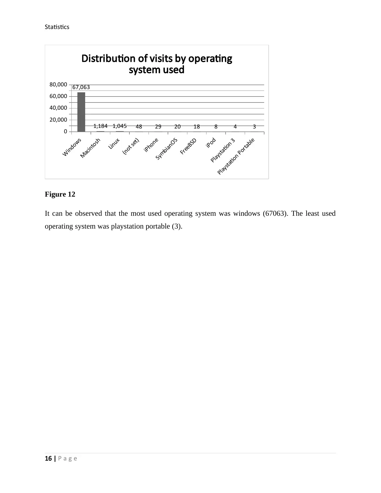
Visits by top 10 operating systems chart.
15 | P a g e
Statistics
Windows
Macintosh
Linux
(not set)
iPhone
SymbianOS
FreeBSD
iPod
Playstation 3
Playstation Portable
0
20,000
40,000
60,000
80,000 67,063
1,184 1,045 48 29 20 18 8 4 3
Distribution of visits by operating
system used
Figure 12
It can be observed that the most used operating system was windows (67063). The least used
operating system was playstation portable (3).
16 | P a g e
1 out of 16
Related Documents
Your All-in-One AI-Powered Toolkit for Academic Success.
+13062052269
info@desklib.com
Available 24*7 on WhatsApp / Email
![[object Object]](/_next/static/media/star-bottom.7253800d.svg)
Unlock your academic potential
© 2024 | Zucol Services PVT LTD | All rights reserved.


