Statistics and Data Modelling Assignment - Desklib

The paper is a study of the transport system in New South Wales, Australia. Data was obtained from the NSW open data for transport from the government site and a sample of the same was used to study the scope of the government to grow and improve upon the scenario as suggested from the data. The opal on and off dataset was used for the purpose of enquiry.

Running head: STATISTICS AND DATA MODELLING ASSIGNMENT
STATISTICS AND DATA MODELLING ASSIGNMENT
Name of Student
Name of University
Author Note

1STATISTICS AND DATA MODELLING ASSIGNMENT
Table of Contents
Section 1: Introduction...............................................................................................................2
Section 2: Analysis of single variable in Dataset 1....................................................................3
a).............................................................................................................................................3
b)............................................................................................................................................5
Section 3: Analysis of two variables in Dataset 1......................................................................6
a).............................................................................................................................................6
b)............................................................................................................................................7
c).............................................................................................................................................8
Section 4: Collect and Analyse Dataset 2..................................................................................8
Section 5: Discussionand Conclusion......................................................................................12
References................................................................................................................................14

2STATISTICS AND DATA MODELLING ASSIGNMENT
Section 1: Introduction
The paper is a study of the transport system in New South Wales, Australia. Data was
obtained from the NSW open data for transport from the government site and a sample of the
same was used to study the scope of the government to grow and improve upon the scenario
as suggested from the data. The opal on and off dataset was used for the purpose of enquiry.
The opal card is an all purpose transport card which can be used for travelling by ferry, light
rail, bus and train by anyone who possess it. It also provides a way to track and keep records
of travel patterns of the passengers for the purpose of further developments as per the
perceived issues and needs (Culnane, Rubinstein and Teague 2017).
Ortega-Tong (2013) conducted a study using smart card data like Opal card in
London, which is the Oyster card. The study used the data to classify passengers on the basis
of frequency of travel and type of traveller, that is whether workers, students or even visitors
who visited for business or leisure. The analysis however that was used was that of cluster
analysis, done on the basis of characteristics relating to spatial variability, socio-demographic
condition, activity patterns and the choice of modes. The clusters were found to represent
and classify passenger behaviour. Four clusters were found which were of visitors visiting for
leisure, visitors visiting for business, registered users who use the mode regularly and those
who use in more occasionally than on a regular basis.
Hence data from smart card transactions have been proved to be useful for
understanding passenger behaviour and pattern. This study focuses on the mode of transport
and the frequency of tapping in and out for the state of NSW in Australia.
Dataset 1 is the sample of data obtained from the Opal Tap on and Tap Off Location-
8th to 14th August 2016 dataset, as available via the Transport or NSW Open Data. The dataset can be

3STATISTICS AND DATA MODELLING ASSIGNMENT
accessed via the link, https://opendata.transport.nsw.gov.au/dataset/opal-tap-on-and-tap-off. It is
therefore a secondary dataset (Creswell and Creswell 2017). The variables in the sample of size 1000
are mode of the data, with four categories, bus, train, ferry and light rail. The data also includes dates
of transactions, in day, month and year. The variable tap recorded that on or off status. The location of
the tap being accessed was also included. These are all categorical data, except the date variable
which is interval. The variable count is interval type, giving the total number of times the tap was on
or off in a certain location on that certain date.
The second dataset was obtained by using a survey method. The data was collected using
simple random sampling from travellers across NSW and hence is primary in nature. The simple
random sampling method is an unbiased sample technique which gives equal chance of inclusion into
the sample to all the members of a population. It is a popular probability sampling technique,
considered for being simple and robust. It however can end up not being able to capture the features
of the population fully if the representation of different factions in the population is not equally
proportionate (Creswell and Creswell 2017). For example if the number of students in the
considered population is lower than the number of workers, then the sample could fail to gather
enough information about the students. Nonetheless, it is proven to work fairly well if proper care is
taken with regard to such complexities. The variables based on which data was collected are, gender,
mode of transportation and the anticipated cost of public transport per month for the individual.
Section 2: Analysis of single variable in Dataset 1
a)
The first research question of interest is regarding the type or mode of transport for
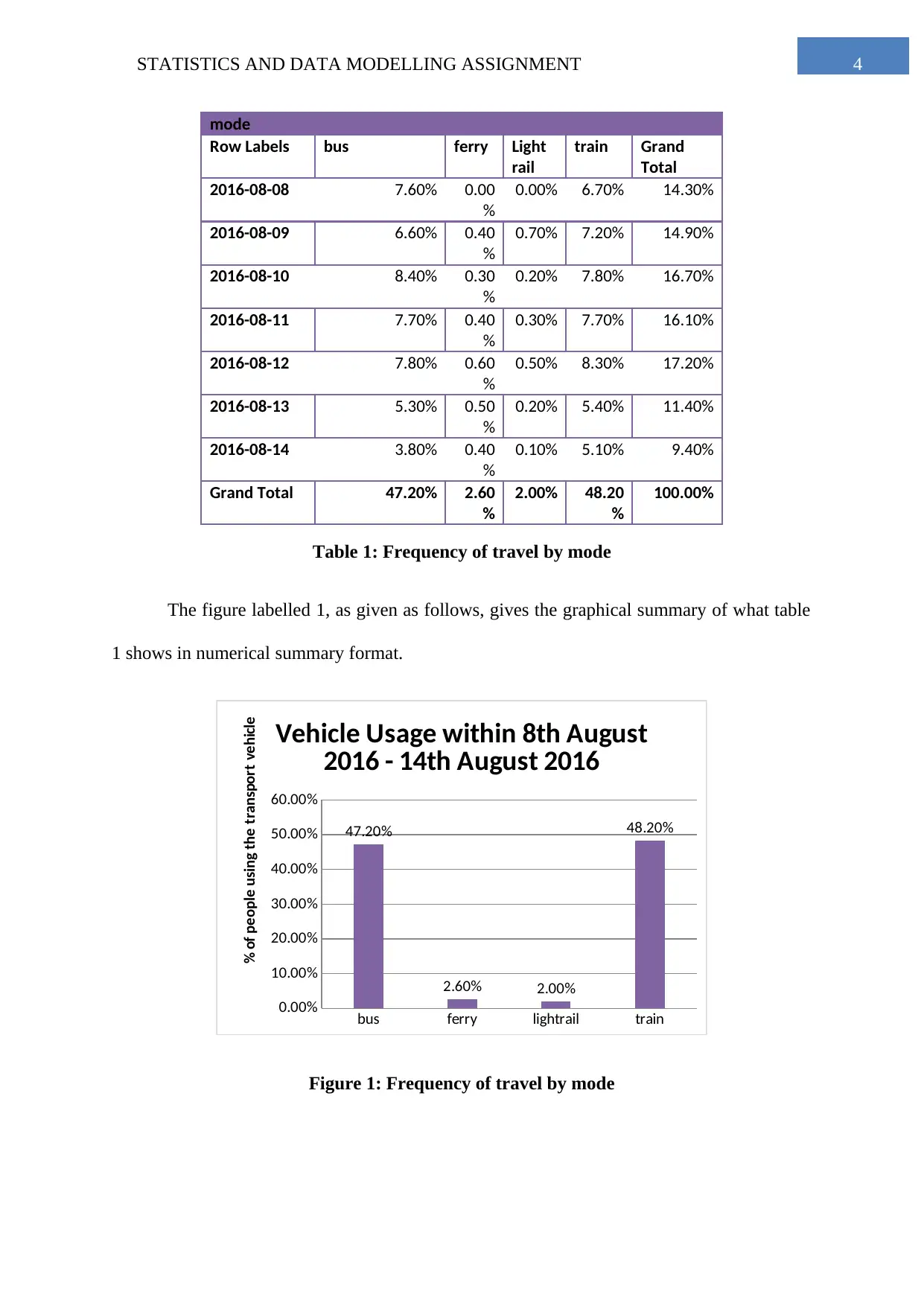
the passengers in the period 8th August , 2016 to 14th August , 2016. The following table,
labelled table 1, gives the numerical summary of the passengers in each mode of transport
within the given time frame.
Count of Column Labels

4STATISTICS AND DATA MODELLING ASSIGNMENT
mode
Row Labels bus ferry Light
rail
train Grand
Total
2016-08-08 7.60% 0.00
%
0.00% 6.70% 14.30%
2016-08-09 6.60% 0.40
%
0.70% 7.20% 14.90%
2016-08-10 8.40% 0.30
%
0.20% 7.80% 16.70%
2016-08-11 7.70% 0.40
%
0.30% 7.70% 16.10%
2016-08-12 7.80% 0.60
%
0.50% 8.30% 17.20%
2016-08-13 5.30% 0.50
%
0.20% 5.40% 11.40%
2016-08-14 3.80% 0.40
%
0.10% 5.10% 9.40%
Grand Total 47.20% 2.60
%
2.00% 48.20
%
100.00%
Table 1: Frequency of travel by mode
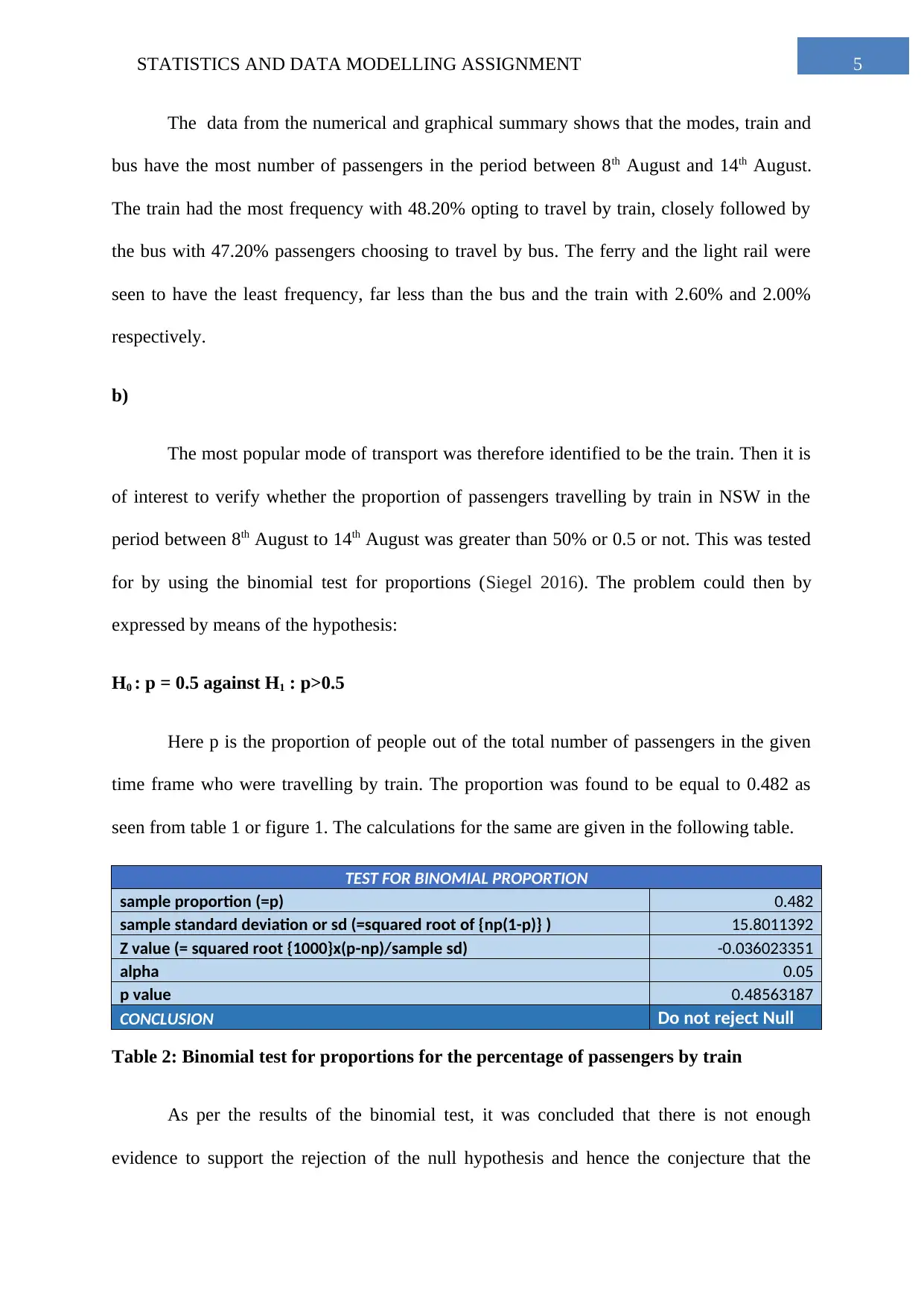
The figure labelled 1, as given as follows, gives the graphical summary of what table
1 shows in numerical summary format.
bus ferry lightrail train
0.00%
10.00%
20.00%
30.00%
40.00%
50.00%
60.00%
47.20%
2.60% 2.00%
48.20%
Vehicle Usage within 8th August
2016 - 14th August 2016
% of people using the transport vehicle
Figure 1: Frequency of travel by mode

5STATISTICS AND DATA MODELLING ASSIGNMENT
The data from the numerical and graphical summary shows that the modes, train and
bus have the most number of passengers in the period between 8th August and 14th August.
The train had the most frequency with 48.20% opting to travel by train, closely followed by
the bus with 47.20% passengers choosing to travel by bus. The ferry and the light rail were
seen to have the least frequency, far less than the bus and the train with 2.60% and 2.00%
respectively.
b)
The most popular mode of transport was therefore identified to be the train. Then it is
of interest to verify whether the proportion of passengers travelling by train in NSW in the
period between 8th August to 14th August was greater than 50% or 0.5 or not. This was tested
for by using the binomial test for proportions (Siegel 2016). The problem could then by
expressed by means of the hypothesis:
H0 : p = 0.5 against H1 : p>0.5
Here p is the proportion of people out of the total number of passengers in the given
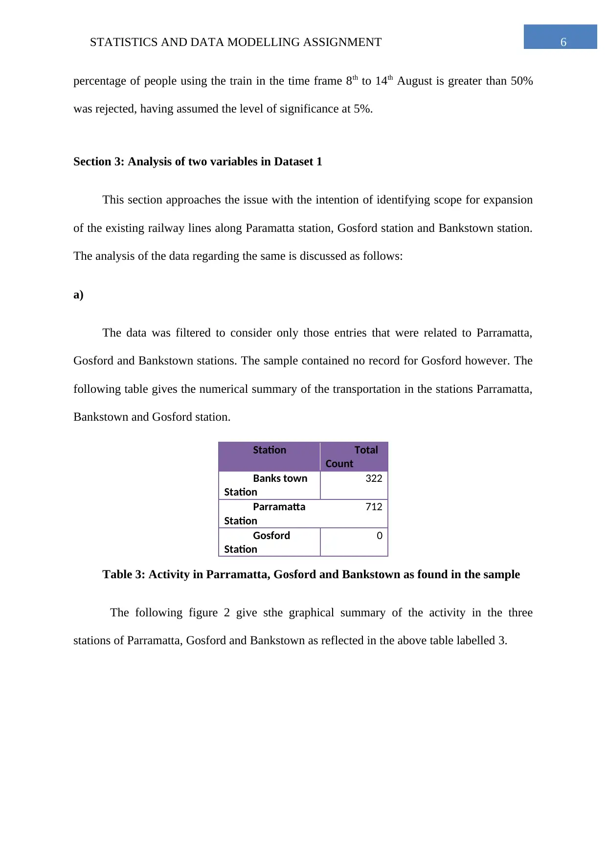
time frame who were travelling by train. The proportion was found to be equal to 0.482 as
seen from table 1 or figure 1. The calculations for the same are given in the following table.
TEST FOR BINOMIAL PROPORTION
sample proportion (=p) 0.482
sample standard deviation or sd (=squared root of {np(1-p)} ) 15.8011392
Z value (= squared root {1000}x(p-np)/sample sd) -0.036023351
alpha 0.05
p value 0.48563187
CONCLUSION Do not reject Null
Table 2: Binomial test for proportions for the percentage of passengers by train
As per the results of the binomial test, it was concluded that there is not enough
evidence to support the rejection of the null hypothesis and hence the conjecture that the

6STATISTICS AND DATA MODELLING ASSIGNMENT
percentage of people using the train in the time frame 8th to 14th August is greater than 50%
was rejected, having assumed the level of significance at 5%.
Section 3: Analysis of two variables in Dataset 1
This section approaches the issue with the intention of identifying scope for expansion
of the existing railway lines along Paramatta station, Gosford station and Bankstown station.
The analysis of the data regarding the same is discussed as follows:
a)
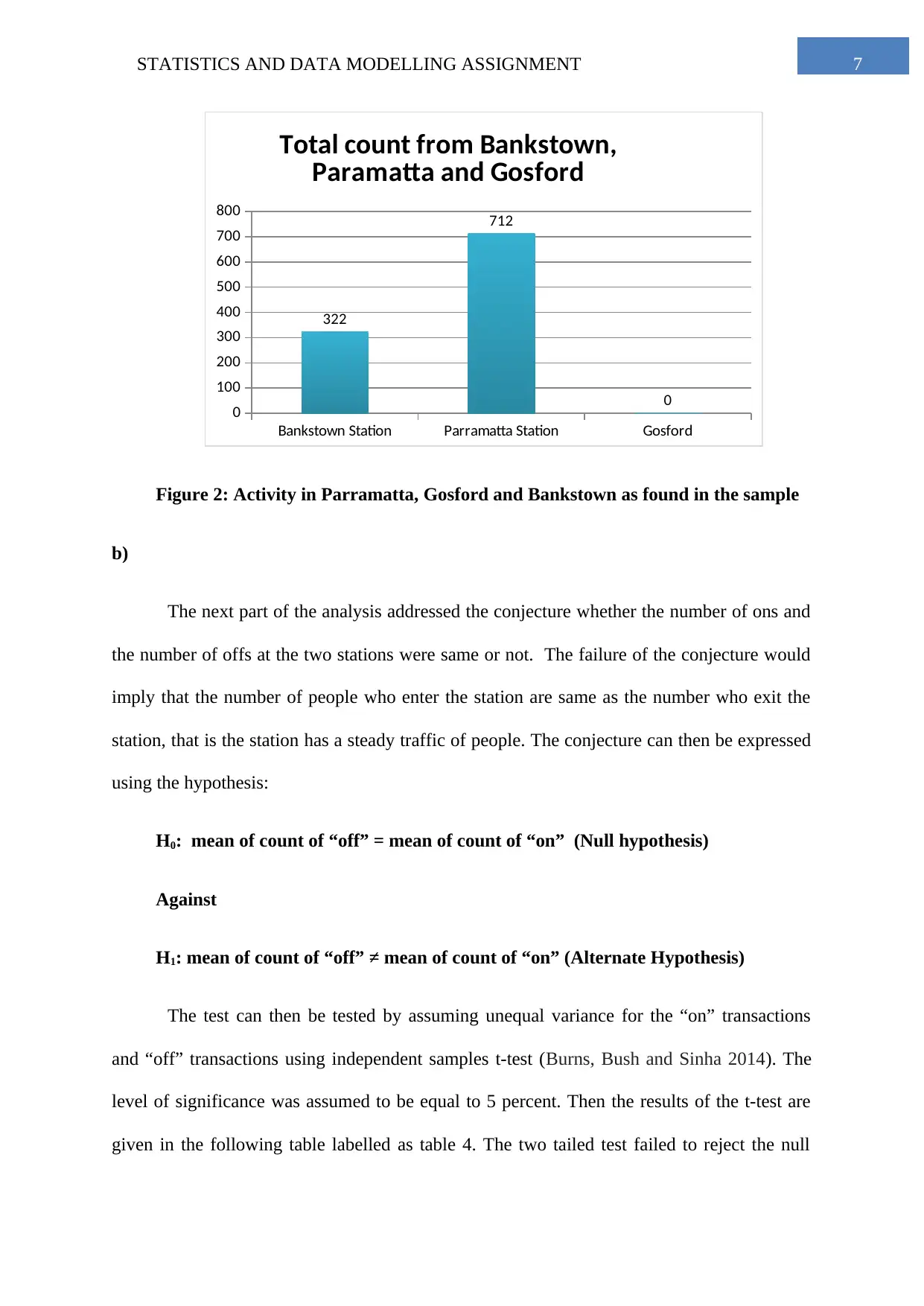
The data was filtered to consider only those entries that were related to Parramatta,
Gosford and Bankstown stations. The sample contained no record for Gosford however. The
following table gives the numerical summary of the transportation in the stations Parramatta,
Bankstown and Gosford station.
Station Total
Count
Banks town
Station
322
Parramatta
Station
712
Gosford
Station
0
Table 3: Activity in Parramatta, Gosford and Bankstown as found in the sample
The following figure 2 give sthe graphical summary of the activity in the three
stations of Parramatta, Gosford and Bankstown as reflected in the above table labelled 3.

7STATISTICS AND DATA MODELLING ASSIGNMENT
Bankstown Station Parramatta Station Gosford
0
100
200
300
400
500
600
700
800
322
712
0
Total count from Bankstown,
Paramatta and Gosford
Figure 2: Activity in Parramatta, Gosford and Bankstown as found in the sample
b)
The next part of the analysis addressed the conjecture whether the number of ons and
the number of offs at the two stations were same or not. The failure of the conjecture would
imply that the number of people who enter the station are same as the number who exit the
station, that is the station has a steady traffic of people. The conjecture can then be expressed
using the hypothesis:
H0: mean of count of “off” = mean of count of “on” (Null hypothesis)
Against
H1: mean of count of “off” ≠ mean of count of “on” (Alternate Hypothesis)
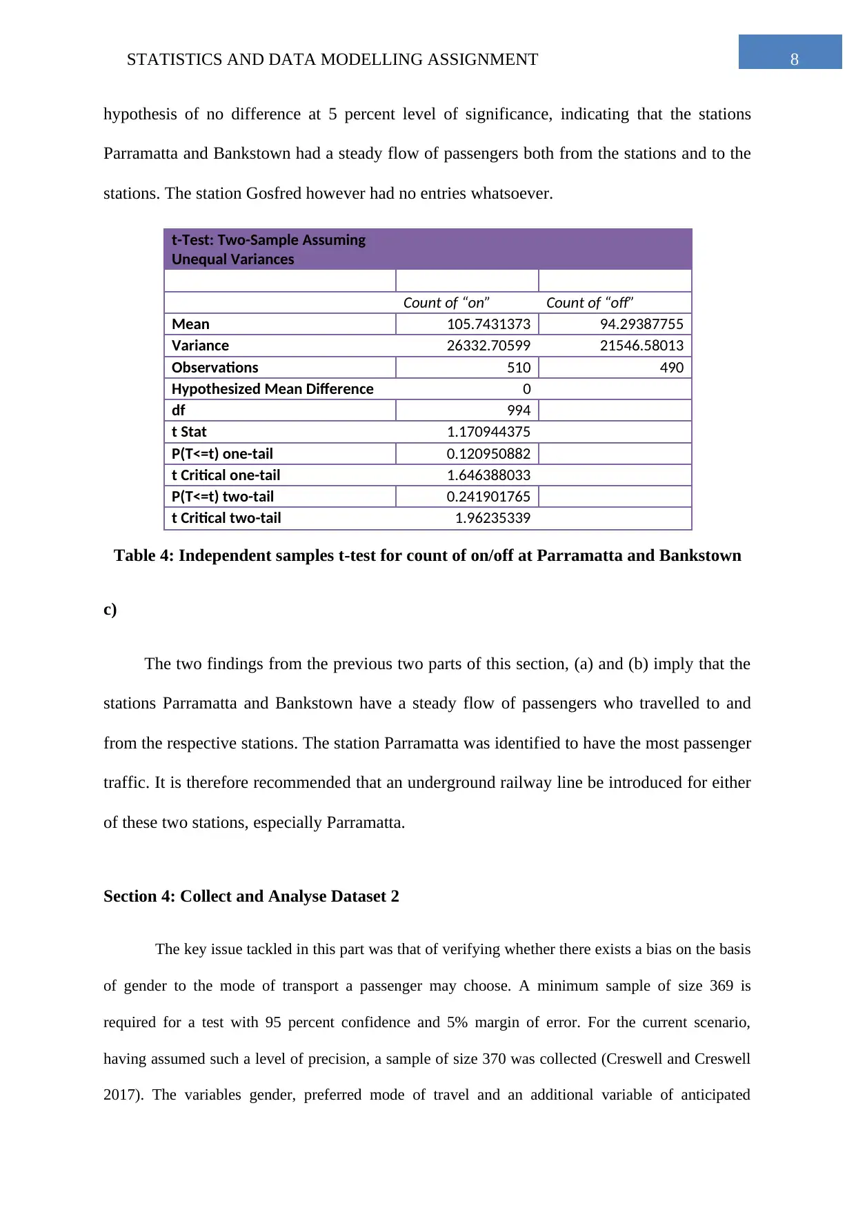
The test can then be tested by assuming unequal variance for the “on” transactions
and “off” transactions using independent samples t-test (Burns, Bush and Sinha 2014). The
level of significance was assumed to be equal to 5 percent. Then the results of the t-test are
given in the following table labelled as table 4. The two tailed test failed to reject the null

8STATISTICS AND DATA MODELLING ASSIGNMENT
hypothesis of no difference at 5 percent level of significance, indicating that the stations
Parramatta and Bankstown had a steady flow of passengers both from the stations and to the
stations. The station Gosfred however had no entries whatsoever.
t-Test: Two-Sample Assuming
Unequal Variances
Count of “on” Count of “off”
Mean 105.7431373 94.29387755
Variance 26332.70599 21546.58013
Observations 510 490
Hypothesized Mean Difference 0
df 994
t Stat 1.170944375
P(T<=t) one-tail 0.120950882
t Critical one-tail 1.646388033
P(T<=t) two-tail 0.241901765
t Critical two-tail 1.96235339
Table 4: Independent samples t-test for count of on/off at Parramatta and Bankstown
c)
The two findings from the previous two parts of this section, (a) and (b) imply that the
stations Parramatta and Bankstown have a steady flow of passengers who travelled to and
from the respective stations. The station Parramatta was identified to have the most passenger
traffic. It is therefore recommended that an underground railway line be introduced for either
of these two stations, especially Parramatta.
Section 4: Collect and Analyse Dataset 2
The key issue tackled in this part was that of verifying whether there exists a bias on the basis
of gender to the mode of transport a passenger may choose. A minimum sample of size 369 is
required for a test with 95 percent confidence and 5% margin of error. For the current scenario,
having assumed such a level of precision, a sample of size 370 was collected (Creswell and Creswell
2017). The variables gender, preferred mode of travel and an additional variable of anticipated

9STATISTICS AND DATA MODELLING ASSIGNMENT
monthly expense on transport was collected by means of a survey from residents of NSW. The
findings of the survey are hence discussed.
50.54%49.46%
Gender Demographics
F M
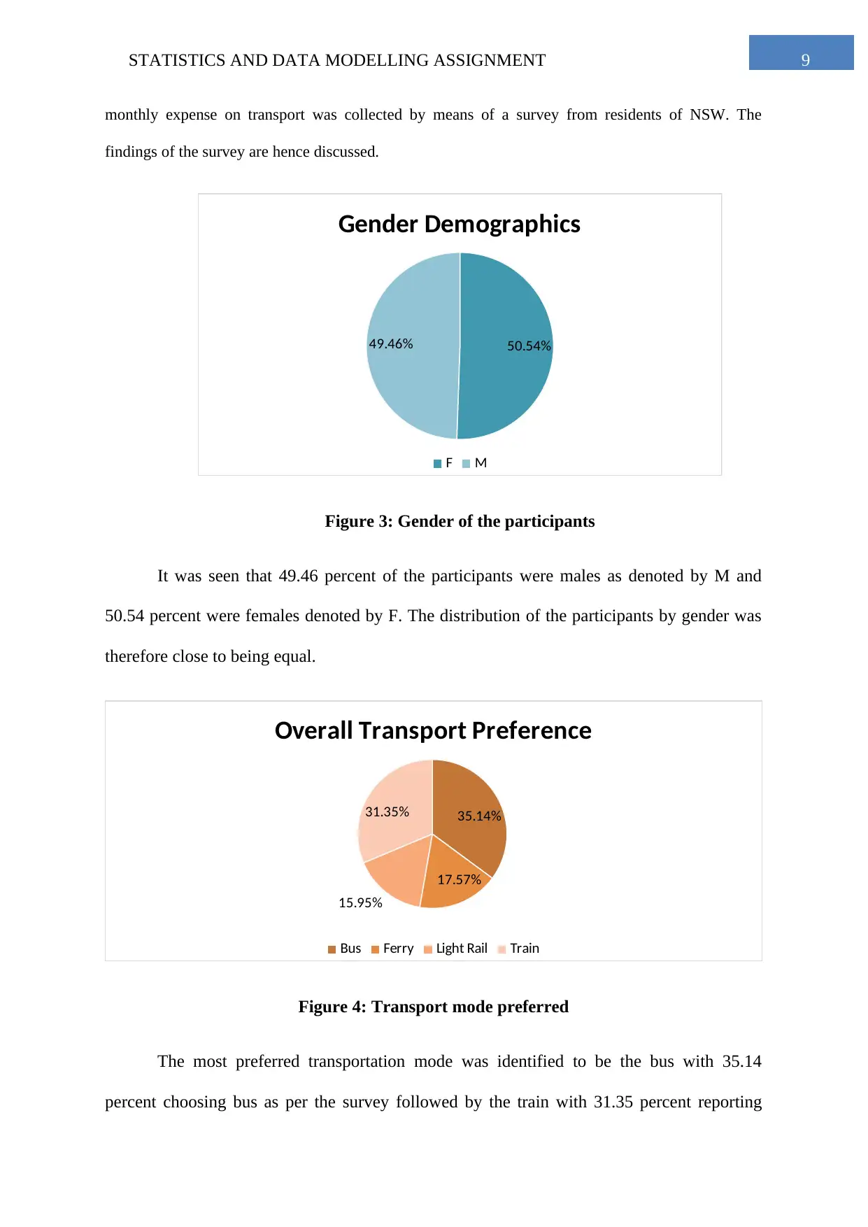
Figure 3: Gender of the participants
It was seen that 49.46 percent of the participants were males as denoted by M and
50.54 percent were females denoted by F. The distribution of the participants by gender was
therefore close to being equal.
35.14%
17.57%
15.95%
31.35%
Overall Transport Preference
Bus Ferry Light Rail Train
Figure 4: Transport mode preferred
The most preferred transportation mode was identified to be the bus with 35.14
percent choosing bus as per the survey followed by the train with 31.35 percent reporting

10STATISTICS AND DATA MODELLING ASSIGNMENT
train as their transport of choice. 15.95 percent said that they preferred the light rail while
17.57 percent chose the Ferry.
bus ferry light rail train
0.00%
10.00%
20.00%
30.00%
40.00%
50.00%
60.00%
70.00%
80.00%
33.16%
17.65% 20.32%
28.88%
37.16%
17.49% 11.48%
33.88%
Prefered Mode of transport by Gender
Male
Female
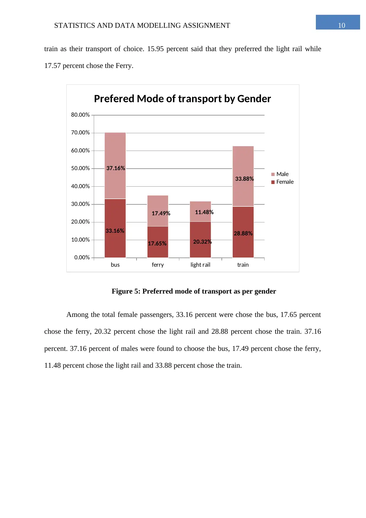
Figure 5: Preferred mode of transport as per gender
Among the total female passengers, 33.16 percent were chose the bus, 17.65 percent
chose the ferry, 20.32 percent chose the light rail and 28.88 percent chose the train. 37.16
percent. 37.16 percent of males were found to choose the bus, 17.49 percent chose the ferry,
11.48 percent chose the light rail and 33.88 percent chose the train.

11STATISTICS AND DATA MODELLING ASSIGNMENT
bus ferry light rail train overall
$-
$20.00
$40.00
$60.00
$80.00
$100.00
$120.00
$140.00
$160.00
$180.00
$200.00
$151.38
$80.77
$91.02
$172.76
$136.05
Expected Earnings per month
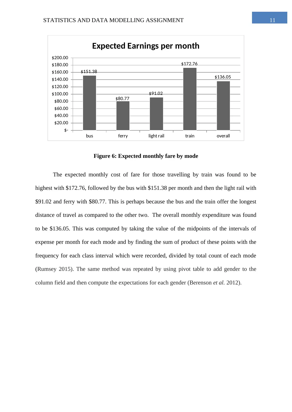
Figure 6: Expected monthly fare by mode
The expected monthly cost of fare for those travelling by train was found to be
highest with $172.76, followed by the bus with $151.38 per month and then the light rail with
$91.02 and ferry with $80.77. This is perhaps because the bus and the train offer the longest
distance of travel as compared to the other two. The overall monthly expenditure was found
to be $136.05. This was computed by taking the value of the midpoints of the intervals of
expense per month for each mode and by finding the sum of product of these points with the
frequency for each class interval which were recorded, divided by total count of each mode
(Rumsey 2015). The same method was repeated by using pivot table to add gender to the
column field and then compute the expectations for each gender (Berenson et al. 2012).

12STATISTICS AND DATA MODELLING ASSIGNMENT
bus ferry light rail train overall
$-
$20.00
$40.00
$60.00
$80.00
$100.00
$120.00
$140.00
$160.00
$180.00
$200.00
$154.84
$86.36
$90.00
$177.78
$127.25
$148.24
$75.00 $92.86
$168.39
$121.12
Expected monthly fare by gender and mode
Female
Male
Figure 7: Expected monthly fare by mode and gender
The findings suggest that the bus is favoured first and the train second by both the
men and the women. However it seems that women prefer the light rail to the ferry whereas
the opposite is seen for the males.
Section 5: Discussionand Conclusion
The study in its analysis of the transport conditions at NSW employed two datasets
one secondary and one primary to explore the possibilities of further development. As per the
secondary data, based on the opal card data available via the transport NSW open data, it is
seen that trains are the most favoured mode of transport followed by the bus. However it was
found that the proportion of people who prefer the train is not greater than 50 percent. The
primary data however suggests that it is actually the bus which is most preferred.
Nonetheless, both the data indicated that the bus and the train are the two most favoured

13STATISTICS AND DATA MODELLING ASSIGNMENT
modes with pretty close preference proportions. The study identified Parramatta and
Bankstown as potential candidates where underground railways could be built. Parramatta
was found to be more suitable however. Using the primary data analysis, among the females,
it was found that bus is the most preferred followed by the train. This was reflected by the
males as well. However the females seemed to prefer the light rail more than the ferry and the
males preferred the ferry over the rail.

14STATISTICS AND DATA MODELLING ASSIGNMENT
References
Berenson, M., Levine, D., Szabat, K.A. and Krehbiel, T.C., 2012. Basic business statistics:
Concepts and applications. Pearson higher education AU.
Burns, A.C., Bush, R.F. and Sinha, N., 2014. Marketing research (Vol. 7). Harlow: Pearson.
Creswell, J.W. and Creswell, J.D., 2017. Research design: Qualitative, quantitative, and
mixed methods approaches. Sage publications.
Culnane, C., Rubinstein, B.I. and Teague, V., 2017. Privacy assessment of de-identified opal
data: A report for transport for NSW. arXiv preprint arXiv:1704.08547.
Ortega-Tong, M.A., 2013. Classification of London's public transport users using smart card
data (Doctoral dissertation, Massachusetts Institute of Technology).
Rumsey, D.J., 2015. U Can: statistics for dummies. John Wiley & Sons.
Siegel, A., 2016. Practical business statistics. Academic Press.