Statistics - Desklib

This article covers topics like frequency distribution, histogram, linear regression, ANOVA, and more in statistics. It includes solved assignments, essays, dissertations, and study material. The article also explains the significance of predictor variables, measures of central tendency, and the coefficient of determination. It concludes with a multiple linear regression analysis of mobile phones sold per day with two predictor variables.

Running head: GROUP ASSIGNMENT – STATISTICS
Statistics
Name
Course Number
Date
Faculty Name

STATISTICS 2
Statistics
1. Frequency distribution and histogram
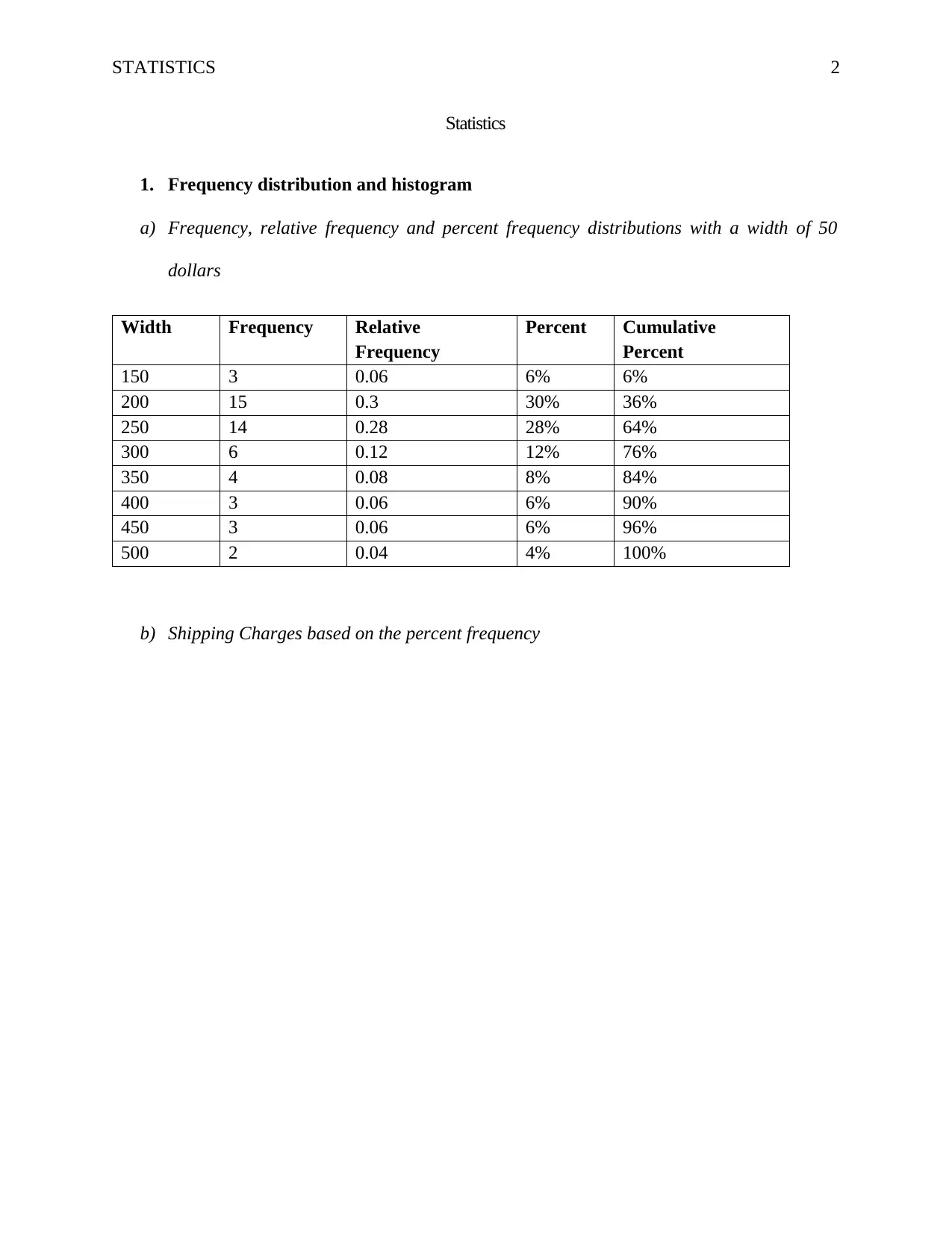
a) Frequency, relative frequency and percent frequency distributions with a width of 50
dollars
Width Frequency Relative
Frequency
Percent Cumulative
Percent
150 3 0.06 6% 6%
200 15 0.3 30% 36%
250 14 0.28 28% 64%
300 6 0.12 12% 76%
350 4 0.08 8% 84%
400 3 0.06 6% 90%
450 3 0.06 6% 96%
500 2 0.04 4% 100%
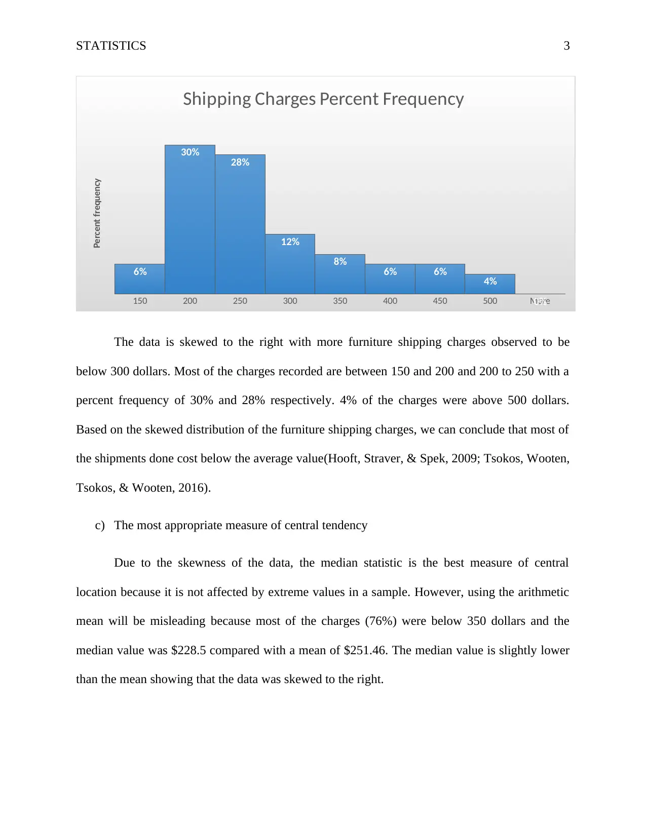
b) Shipping Charges based on the percent frequency

STATISTICS 3
150 200 250 300 350 400 450 500 More
6%
30% 28%
12%
8% 6% 6% 4%
0%
Shipping Charges Percent Frequency
Percent frequency
The data is skewed to the right with more furniture shipping charges observed to be
below 300 dollars. Most of the charges recorded are between 150 and 200 and 200 to 250 with a
percent frequency of 30% and 28% respectively. 4% of the charges were above 500 dollars.
Based on the skewed distribution of the furniture shipping charges, we can conclude that most of
the shipments done cost below the average value(Hooft, Straver, & Spek, 2009; Tsokos, Wooten,
Tsokos, & Wooten, 2016).
c) The most appropriate measure of central tendency
Due to the skewness of the data, the median statistic is the best measure of central
location because it is not affected by extreme values in a sample. However, using the arithmetic
mean will be misleading because most of the charges (76%) were below 350 dollars and the
median value was $228.5 compared with a mean of $251.46. The median value is slightly lower
than the mean showing that the data was skewed to the right.

STATISTICS 4
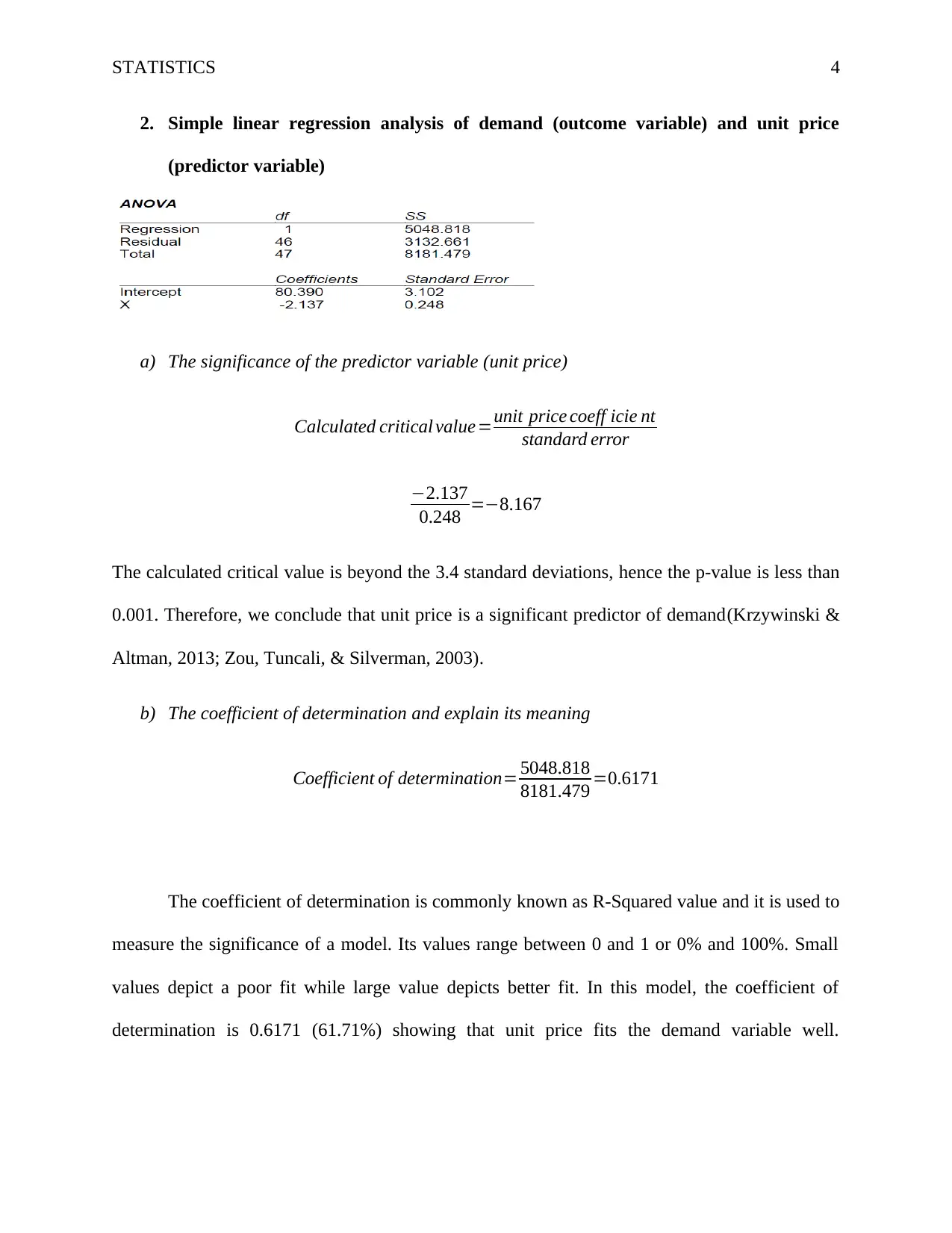
2. Simple linear regression analysis of demand (outcome variable) and unit price
(predictor variable)
a) The significance of the predictor variable (unit price)
Calculated critical value=unit price coeff icie nt
standard error
−2.137
0.248 =−8.167
The calculated critical value is beyond the 3.4 standard deviations, hence the p-value is less than
0.001. Therefore, we conclude that unit price is a significant predictor of demand(Krzywinski &
Altman, 2013; Zou, Tuncali, & Silverman, 2003).
b) The coefficient of determination and explain its meaning
Coefficient of determination= 5048.818
8181.479 =0.6171
The coefficient of determination is commonly known as R-Squared value and it is used to
measure the significance of a model. Its values range between 0 and 1 or 0% and 100%. Small
values depict a poor fit while large value depicts better fit. In this model, the coefficient of
determination is 0.6171 (61.71%) showing that unit price fits the demand variable well.

STATISTICS 5
Therefore, 61.71% of the variation in demand for a product is explained by its price(Roberts,
2013).
c) Coefficient of correlation
The square root of the R-squared value gives the coefficient of determination which runs
between -1 to +1. Negatives indicate a negative relationship while positives show a positive
correlation between variables.
√ 0.6171=0.786
According to the calculated coefficient of determination, it shows that there is a strong
positive relationship between unit price and demand. Although we could not determine whether
the correlation is positive or negative, the model output can determine the nature of the
relationship by checking the sign of the predictor coefficient, which was positive.

STATISTICS 6
3. A study design with three treatments (One-way ANOVA)
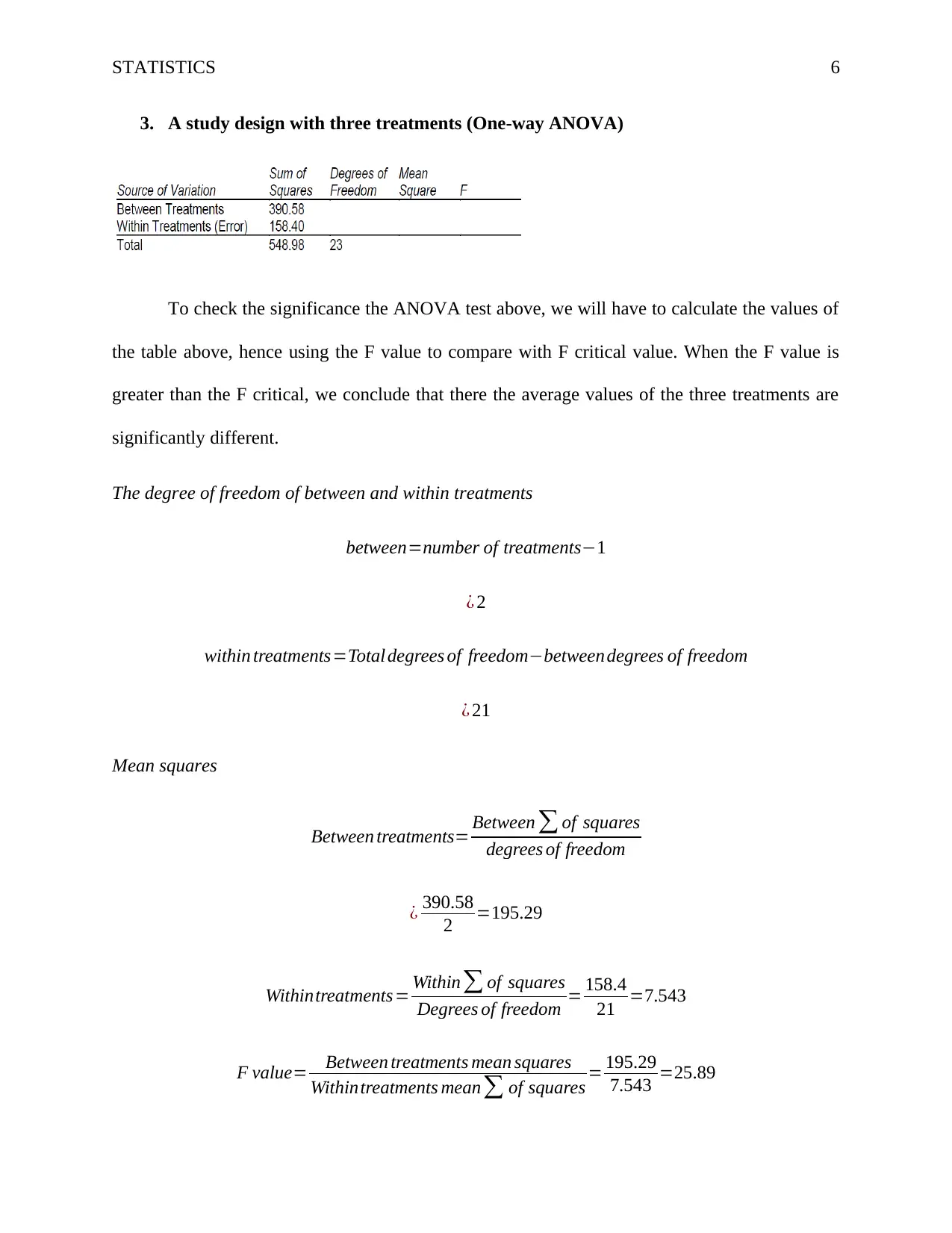
To check the significance the ANOVA test above, we will have to calculate the values of
the table above, hence using the F value to compare with F critical value. When the F value is
greater than the F critical, we conclude that there the average values of the three treatments are
significantly different.
The degree of freedom of between and within treatments
between=number of treatments−1
¿ 2
within treatments=Total degrees of freedom−between degrees of freedom
¿ 21
Mean squares
Between treatments= Between ∑ of squares
degrees of freedom
¿ 390.58
2 =195.29
Withintreatments= Within∑ of squares
Degrees of freedom = 158.4
21 =7.543
F value= Between treatments mean squares
Withintreatments mean∑ of squares = 195.29
7.543 =25.89

STATISTICS 7
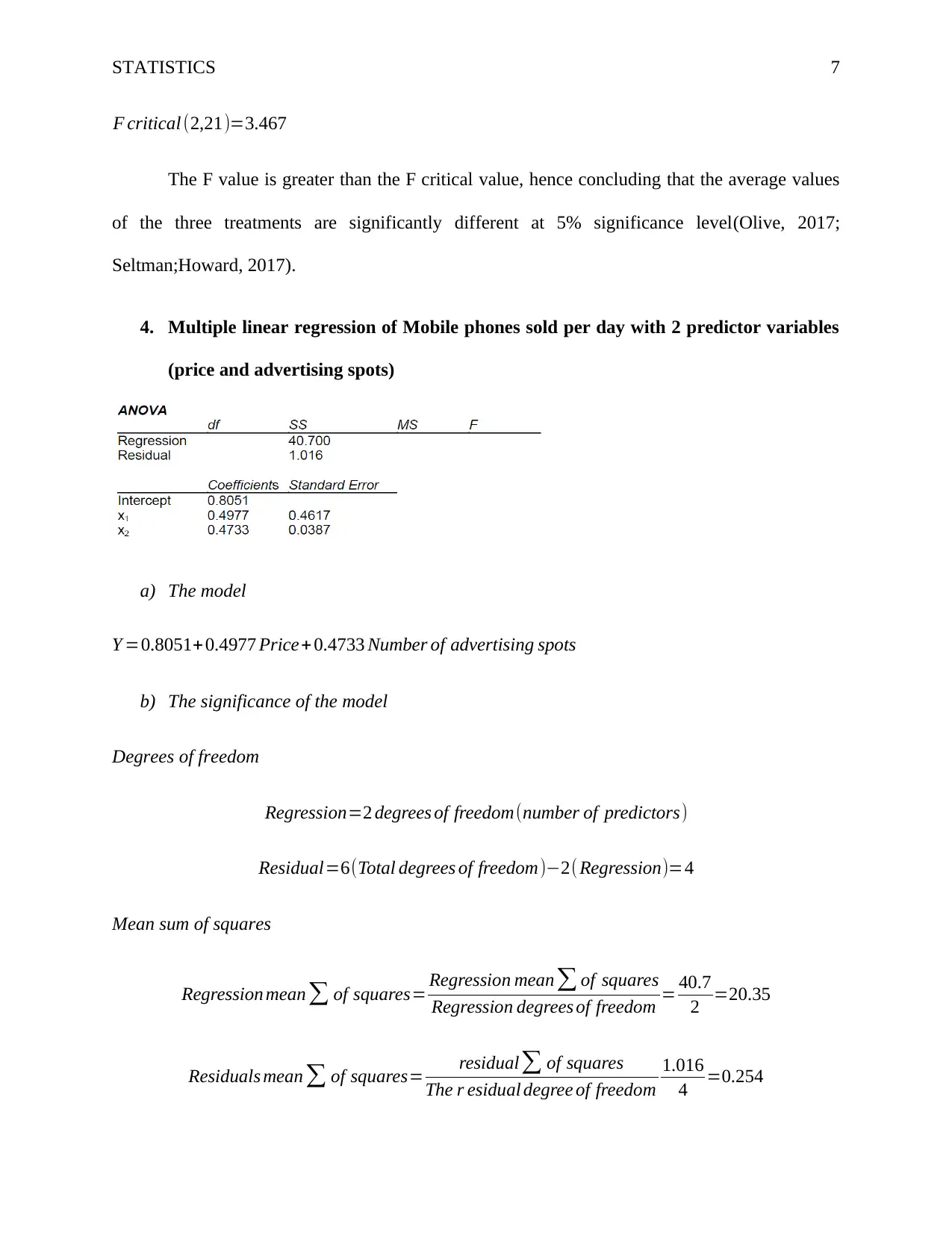
F critical (2,21)=3.467
The F value is greater than the F critical value, hence concluding that the average values
of the three treatments are significantly different at 5% significance level(Olive, 2017;
Seltman;Howard, 2017).
4. Multiple linear regression of Mobile phones sold per day with 2 predictor variables
(price and advertising spots)
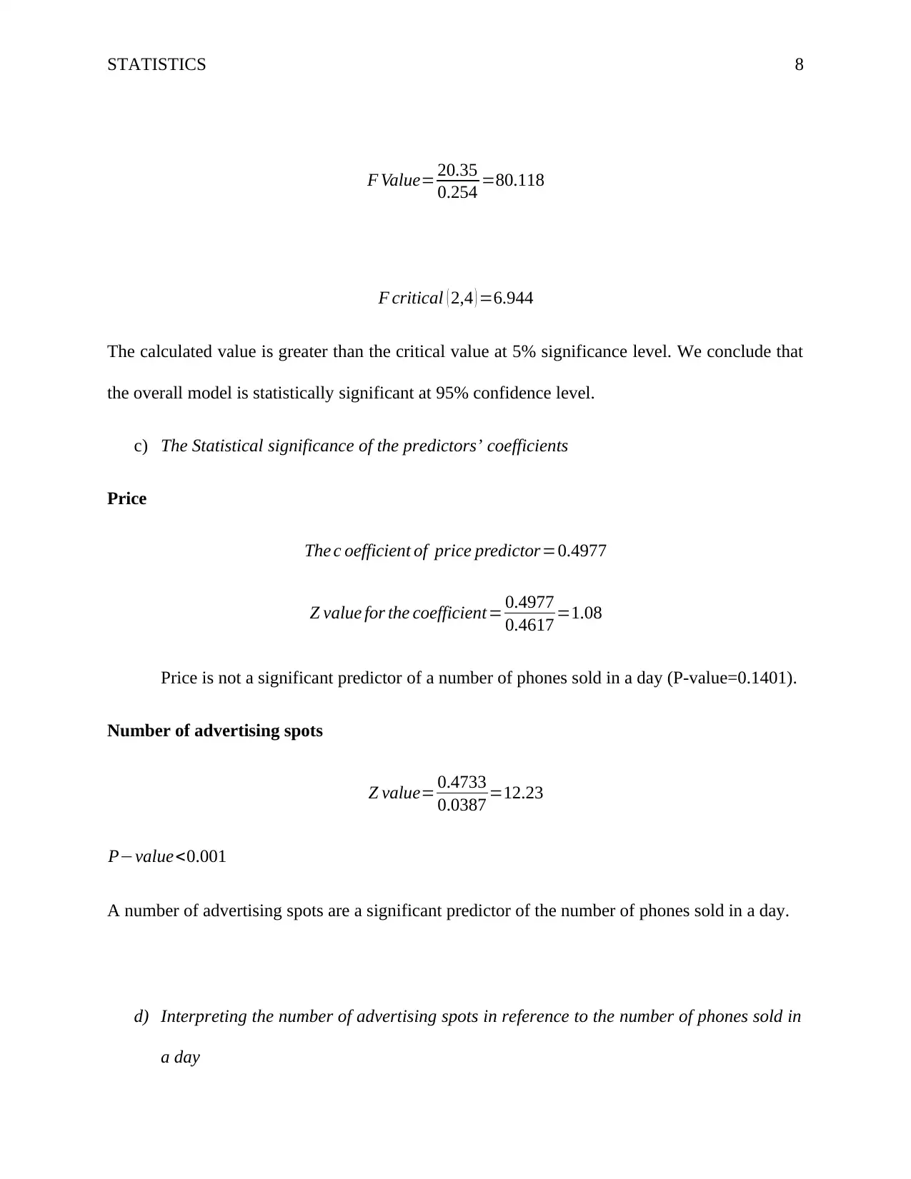
a) The model
Y =0.8051+0.4977 Price+ 0.4733 Number of advertising spots
b) The significance of the model
Degrees of freedom
Regression=2 degrees of freedom(number of predictors)
Residual=6(Total degrees of freedom)−2( Regression)=4
Mean sum of squares
Regression mean∑ of squares= Regression mean∑ of squares
Regression degrees of freedom = 40.7
2 =20.35
Residuals mean ∑ of squares= residual∑ of squares
The r esidual degree of freedom
1.016
4 =0.254

STATISTICS 8
F Value= 20.35
0.254 =80.118
F critical ( 2,4 ) =6.944
The calculated value is greater than the critical value at 5% significance level. We conclude that
the overall model is statistically significant at 95% confidence level.
c) The Statistical significance of the predictors’ coefficients
Price
The c oefficient of price predictor=0.4977
Z value for the coefficient= 0.4977
0.4617 =1.08
Price is not a significant predictor of a number of phones sold in a day (P-value=0.1401).
Number of advertising spots
Z value= 0.4733
0.0387 =12.23
P−value<0.001
A number of advertising spots are a significant predictor of the number of phones sold in a day.
d) Interpreting the number of advertising spots in reference to the number of phones sold in
a day

STATISTICS 9
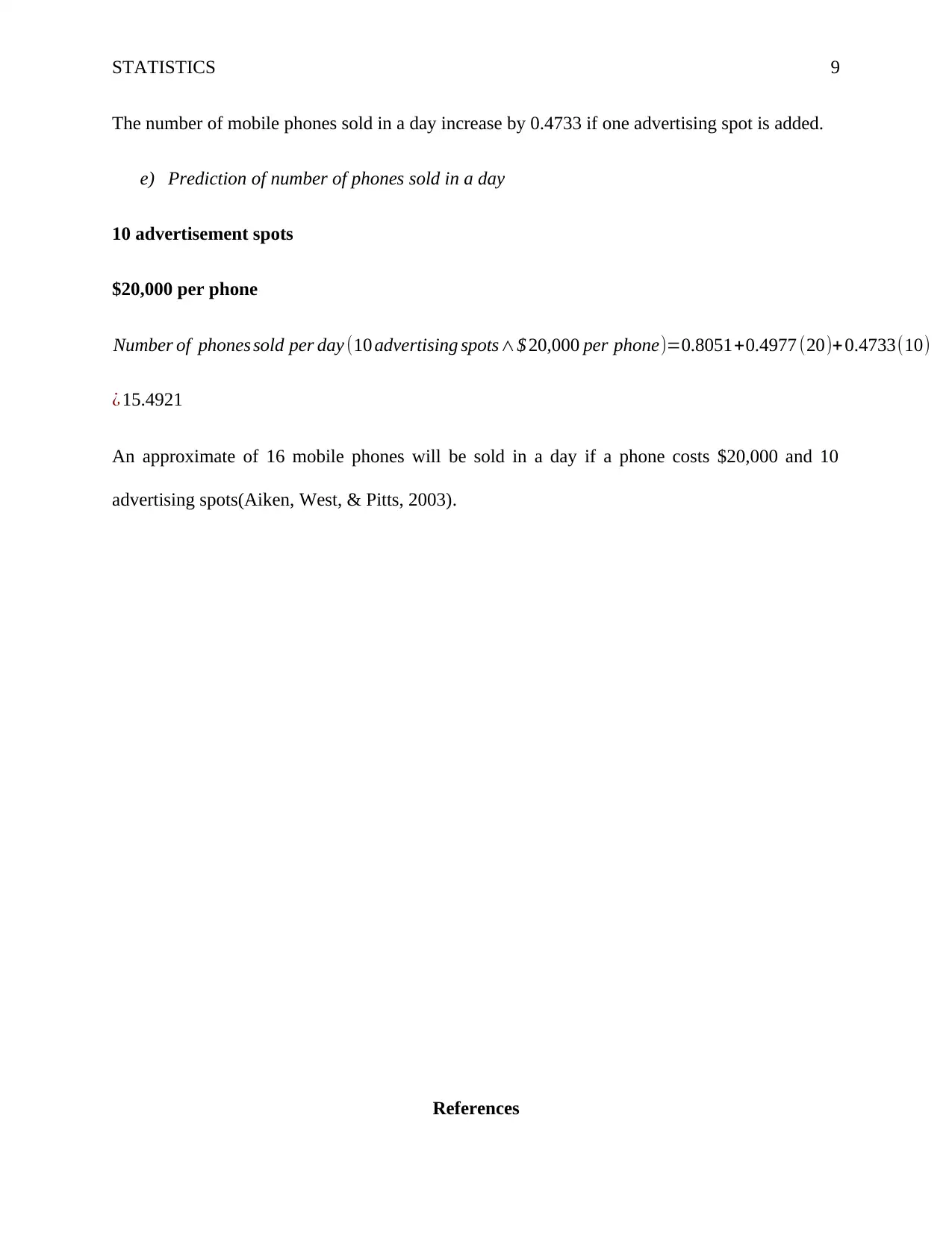
The number of mobile phones sold in a day increase by 0.4733 if one advertising spot is added.
e) Prediction of number of phones sold in a day
10 advertisement spots
$20,000 per phone
Number of phones sold per day (10 advertising spots∧$ 20,000 per phone)=0.8051+0.4977 (20)+ 0.4733(10)
¿ 15.4921
An approximate of 16 mobile phones will be sold in a day if a phone costs $20,000 and 10
advertising spots(Aiken, West, & Pitts, 2003).
References

STATISTICS 10
Aiken, L. S., West, S. G., & Pitts, S. C. (2003). Multiple Linear Regression. Handbook of
Psychology, 481–507. https://doi.org/10.1051/eas/1466005
Hooft, R. W. W., Straver, L. H., & Spek, A. L. (2009). Probability plots based on Student’s t-
distribution. Acta Crystallographica Section A: Foundations of Crystallography, 65(4),
319–321. https://doi.org/10.1107/S0108767309009908
Krzywinski, M., & Altman, N. (2013). Points of significance: Significance, P values and t-tests.
Nature Methods. https://doi.org/10.1038/nmeth.2698
Olive, D. J. (2017). One Way Anova. In Linear Regression (pp. 175–211).
https://doi.org/10.1007/978-3-319-55252-1_5
Roberts, D. (2013). Statistics 2 - Correlation Coefficient and Coefficient of Determination.
Retrieved from http://mathbits.com/MathBits/TISection/Statistics2/correlation.htm
Seltman;Howard. (2017). One-Way ANOVA. Experimental Design and Analysis, 171–190.
Retrieved from https://www.jmp.com/content/dam/jmp/documents/en/academic/learning-
library/04-one-way-anova.pdf
Tsokos, C., Wooten, R., Tsokos, C., & Wooten, R. (2016). Normal Probability. In The Joy of
Finite Mathematics (pp. 231–263). https://doi.org/10.1016/B978-0-12-802967-1.00007-3
Zou, K. H., Tuncali, K., & Silverman, S. G. (2003). Correlation and Simple Linear Regression.
Radiology, 227(3), 617–628. https://doi.org/10.1148/radiol.2273011499