Statistical Analysis of Real Estate Data: A Business Statistics Report

This report presents a statistical analysis of the Adelaide real estate market, utilizing data from 2017 and 2018. The analysis begins with descriptive statistics to examine house prices, including mean, standard deviation, median, and distribution characteristics. The report then applies z-scores to understand individual house prices relative to the mean, followed by a chi-square test to assess the distribution of houses sold across different suburbs. Normal distribution is used to calculate probabilities related to house prices. Furthermore, the report conducts hypothesis tests to evaluate whether the mean selling price equaled a specific value and whether the mean selling prices for 2017 and 2018 were equivalent. The findings provide insights into market trends, price distributions, and the validity of specific assumptions regarding house prices within the Adelaide real estate market.

Running Head: STATISTICS FOR BUSINESS
Statistics for Business
Name of the Student
Name of the University
Author Note

1STATISTICS FOR BUSINESS
Table of Contents
Abstract............................................................................................................................................2
Introduction......................................................................................................................................3
Descriptive Statistics...................................................................................................................3
z-Scores........................................................................................................................................4
Chi-square test.............................................................................................................................5
Normal Distribution.....................................................................................................................6
Section a.......................................................................................................................................7
Section b......................................................................................................................................7
Section c.......................................................................................................................................7
Hypothesis Test I.........................................................................................................................8
Hypothesis Test II........................................................................................................................9
Conclusion.....................................................................................................................................10

2STATISTICS FOR BUSINESS
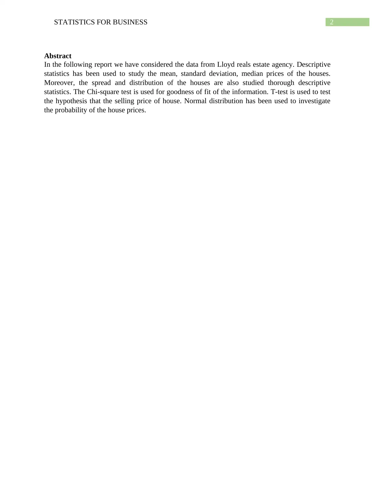
Abstract
In the following report we have considered the data from Lloyd reals estate agency. Descriptive
statistics has been used to study the mean, standard deviation, median prices of the houses.
Moreover, the spread and distribution of the houses are also studied thorough descriptive
statistics. The Chi-square test is used for goodness of fit of the information. T-test is used to test
the hypothesis that the selling price of house. Normal distribution has been used to investigate
the probability of the house prices.

3STATISTICS FOR BUSINESS
Introduction
This report explains the meaning behind the statistical data that was collected by The Lloyd real
estate agency. The Lloyd real estate agency is involved in retail selling of houses at Adelaide.
Information regarding the number of houses sold by the agency in difference suburbs of
Adelaide were collected from the organization. The information pertains to the number of houses
sold and their average prices for a particular suburb. Information for the year 2017 and 2018
were collected from the agency.
For the analysis of the prices of the houses initially the descriptive statistics of the prices is
undertaken. We extend the descriptive statistics to investigate the distribution of the prices.
Further we test whether the number of houses sold in every suburb of Adelaide. Finally, we test
the prices of the houses.
Body
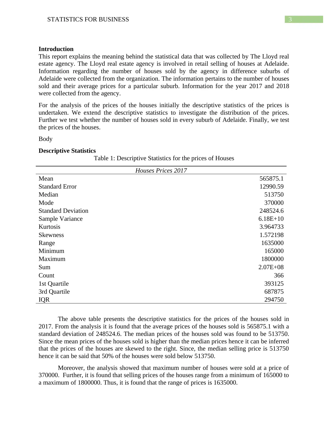
Descriptive Statistics
Table 1: Descriptive Statistics for the prices of Houses
Houses Prices 2017
Mean 565875.1
Standard Error 12990.59
Median 513750
Mode 370000
Standard Deviation 248524.6
Sample Variance 6.18E+10
Kurtosis 3.964733
Skewness 1.572198
Range 1635000
Minimum 165000
Maximum 1800000
Sum 2.07E+08
Count 366
1st Quartile 393125
3rd Quartile 687875
IQR 294750
The above table presents the descriptive statistics for the prices of the houses sold in
2017. From the analysis it is found that the average prices of the houses sold is 565875.1 with a
standard deviation of 248524.6. The median prices of the houses sold was found to be 513750.
Since the mean prices of the houses sold is higher than the median prices hence it can be inferred
that the prices of the houses are skewed to the right. Since, the median selling price is 513750
hence it can be said that 50% of the houses were sold below 513750.
Moreover, the analysis showed that maximum number of houses were sold at a price of
370000. Further, it is found that selling prices of the houses range from a minimum of 165000 to
a maximum of 1800000. Thus, it is found that the range of prices is 1635000.

4STATISTICS FOR BUSINESS
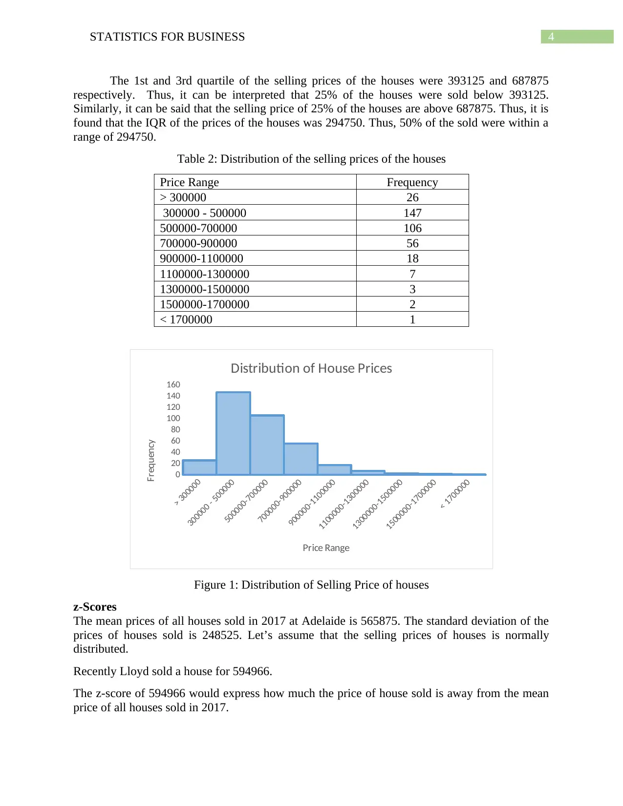
The 1st and 3rd quartile of the selling prices of the houses were 393125 and 687875
respectively. Thus, it can be interpreted that 25% of the houses were sold below 393125.
Similarly, it can be said that the selling price of 25% of the houses are above 687875. Thus, it is
found that the IQR of the prices of the houses was 294750. Thus, 50% of the sold were within a
range of 294750.
Table 2: Distribution of the selling prices of the houses
Price Range Frequency
> 300000 26
300000 - 500000 147
500000-700000 106
700000-900000 56
900000-1100000 18
1100000-1300000 7
1300000-1500000 3
1500000-1700000 2
< 1700000 1
> 300000
300000 - 500000
500000-700000
700000-900000
900000-1100000
1100000-1300000
1300000-1500000
1500000-1700000
< 1700000
0
20
40
60
80
100
120
140
160
Distribution of House Prices
Price Range
Frequency
Figure 1: Distribution of Selling Price of houses
z-Scores
The mean prices of all houses sold in 2017 at Adelaide is 565875. The standard deviation of the
prices of houses sold is 248525. Let’s assume that the selling prices of houses is normally
distributed.
Recently Lloyd sold a house for 594966.
The z-score of 594966 would express how much the price of house sold is away from the mean
price of all houses sold in 2017.

5STATISTICS FOR BUSINESS
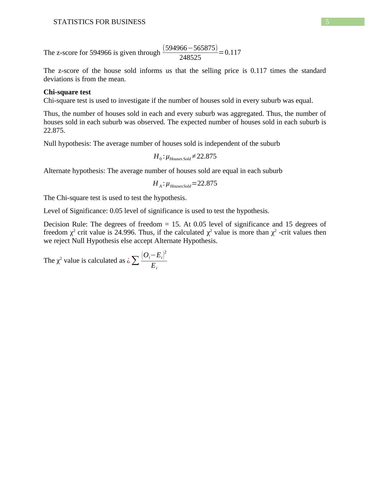
The z-score for 594966 is given through (594966−565875)
248525 =0.117
The z-score of the house sold informs us that the selling price is 0.117 times the standard
deviations is from the mean.
Chi-square test
Chi-square test is used to investigate if the number of houses sold in every suburb was equal.
Thus, the number of houses sold in each and every suburb was aggregated. Thus, the number of
houses sold in each suburb was observed. The expected number of houses sold in each suburb is
22.875.
Null hypothesis: The average number of houses sold is independent of the suburb
H0 : μHouses Sold ≠ 22.875
Alternate hypothesis: The average number of houses sold are equal in each suburb
H A : μHousesSold=22.875
The Chi-square test is used to test the hypothesis.
Level of Significance: 0.05 level of significance is used to test the hypothesis.
Decision Rule: The degrees of freedom = 15. At 0.05 level of significance and 15 degrees of
freedom χ2 crit value is 24.996. Thus, if the calculated χ2 value is more than χ2 -crit values then
we reject Null Hypothesis else accept Alternate Hypothesis.
The χ2 value is calculated as ¿ ∑ ( Oi−Ei ) 2
Ei

6STATISTICS FOR BUSINESS
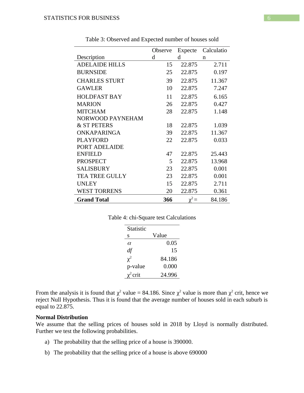
Table 3: Observed and Expected number of houses sold
Description
Observe
d
Expecte
d
Calculatio
n
ADELAIDE HILLS 15 22.875 2.711
BURNSIDE 25 22.875 0.197
CHARLES STURT 39 22.875 11.367
GAWLER 10 22.875 7.247
HOLDFAST BAY 11 22.875 6.165
MARION 26 22.875 0.427
MITCHAM 28 22.875 1.148
NORWOOD PAYNEHAM
& ST PETERS 18 22.875 1.039
ONKAPARINGA 39 22.875 11.367
PLAYFORD 22 22.875 0.033
PORT ADELAIDE
ENFIELD 47 22.875 25.443
PROSPECT 5 22.875 13.968
SALISBURY 23 22.875 0.001
TEA TREE GULLY 23 22.875 0.001
UNLEY 15 22.875 2.711
WEST TORRENS 20 22.875 0.361
Grand Total 366 χ2 = 84.186
Table 4: chi-Square test Calculations
Statistic
s Value
 0.05
df 15
χ2 84.186
p-value 0.000
χ2 crit 24.996
From the analysis it is found that χ2 value = 84.186. Since χ2 value is more than χ2 crit, hence we
reject Null Hypothesis. Thus it is found that the average number of houses sold in each suburb is
equal to 22.875.
Normal Distribution
We assume that the selling prices of houses sold in 2018 by Lloyd is normally distributed.
Further we test the following probabilities.
a) The probability that the selling price of a house is 390000.
b) The probability that the selling price of a house is above 690000

7STATISTICS FOR BUSINESS
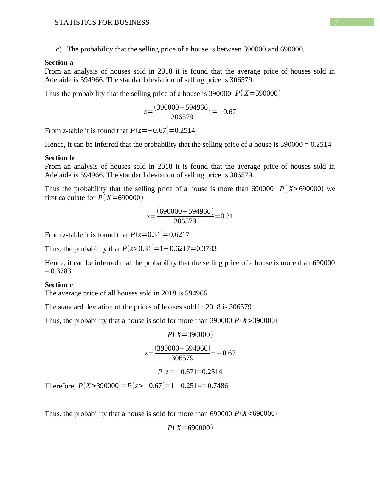
c) The probability that the selling price of a house is between 390000 and 690000.
Section a
From an analysis of houses sold in 2018 it is found that the average price of houses sold in
Adelaide is 594966. The standard deviation of selling price is 306579.
Thus the probability that the selling price of a house is 390000 P( X=390000)
z=(390000−594966)
306579 =−0.67
From z-table it is found that P ( z=−0.67 )=0.2514
Hence, it can be inferred that the probability that the selling price of a house is 390000 = 0.2514
Section b
From an analysis of houses sold in 2018 it is found that the average price of houses sold in
Adelaide is 594966. The standard deviation of selling price is 306579.
Thus the probability that the selling price of a house is more than 690000 P( X> 690000) we
first calculate for P( X=690000)
z=(690000−594966)
306579 =0.31
From z-table it is found that P ( z=0.31 ) =0.6217
Thus, the probability that P ( z> 0.31 )=1−0.6217=0.3783
Hence, it can be inferred that the probability that the selling price of a house is more than 690000
= 0.3783
Section c
The average price of all houses sold in 2018 is 594966
The standard deviation of the prices of houses sold in 2018 is 306579
Thus, the probability that a house is sold for more than 390000 P ( X >390000 )
P( X=390000)
z= ( 390000−594966 )
306579 =−0.67
P ( z=−0.67 ) =0.2514
Therefore, P ( X >390000 )=P ( z >−0.67 )=1−0.2514=0.7486
Thus, the probability that a house is sold for more than 690000 P ( X <690000 )
P( X=690000)

8STATISTICS FOR BUSINESS
z= ( 690000−594966 )
306579 =0.31
P ( z=0.31 ) =0.6217
Therefore, P ( X <690000 ) =P ( z <0.31 ) =1−0.6217=0.3783
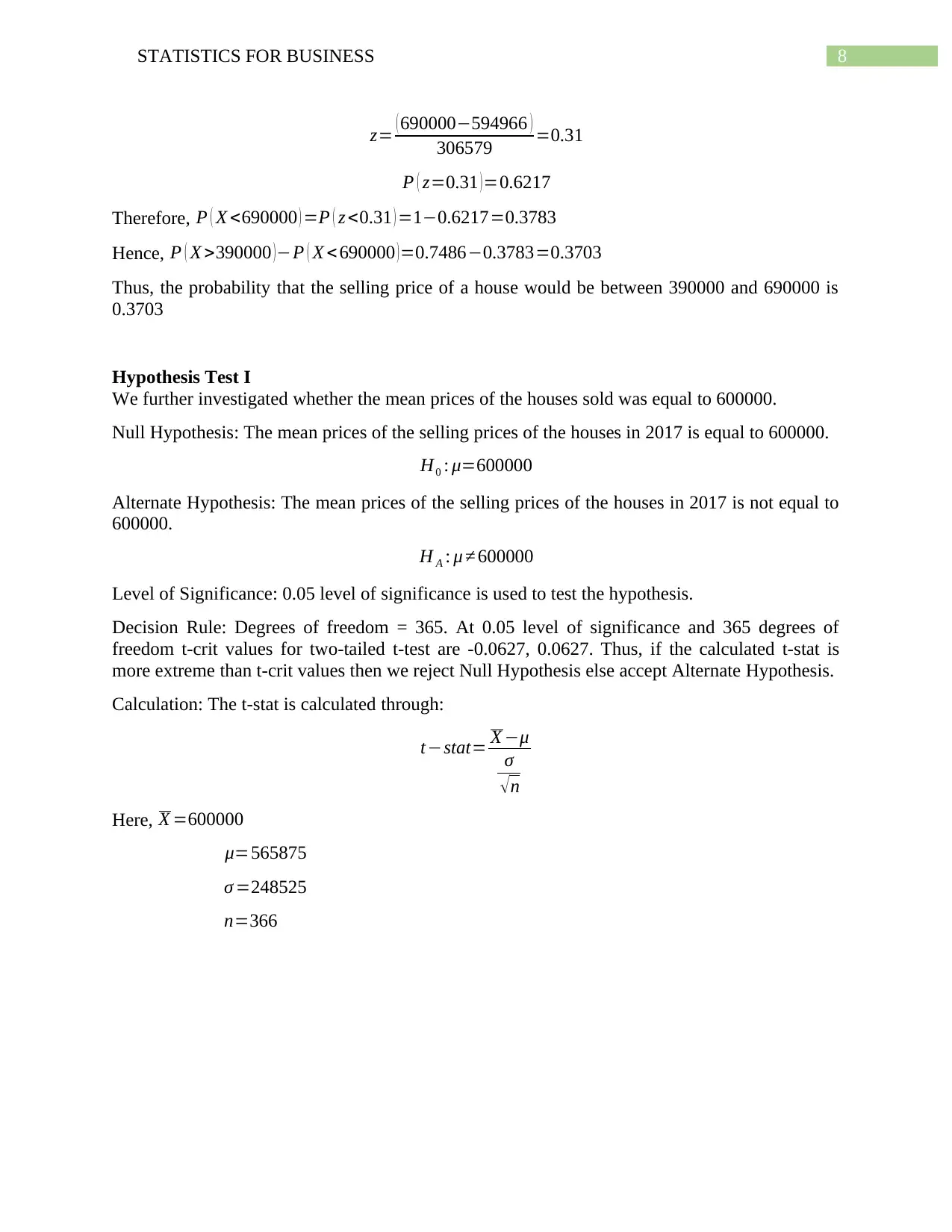
Hence, P ( X >390000 )−P ( X < 690000 )=0.7486−0.3783=0.3703
Thus, the probability that the selling price of a house would be between 390000 and 690000 is
0.3703
Hypothesis Test I
We further investigated whether the mean prices of the houses sold was equal to 600000.
Null Hypothesis: The mean prices of the selling prices of the houses in 2017 is equal to 600000.
H0 : μ=600000
Alternate Hypothesis: The mean prices of the selling prices of the houses in 2017 is not equal to
600000.
H A : μ ≠ 600000
Level of Significance: 0.05 level of significance is used to test the hypothesis.
Decision Rule: Degrees of freedom = 365. At 0.05 level of significance and 365 degrees of
freedom t-crit values for two-tailed t-test are -0.0627, 0.0627. Thus, if the calculated t-stat is
more extreme than t-crit values then we reject Null Hypothesis else accept Alternate Hypothesis.
Calculation: The t-stat is calculated through:
t−stat= X −μ
σ
√n
Here, X =600000
μ=565875
σ =248525
n=366

9STATISTICS FOR BUSINESS
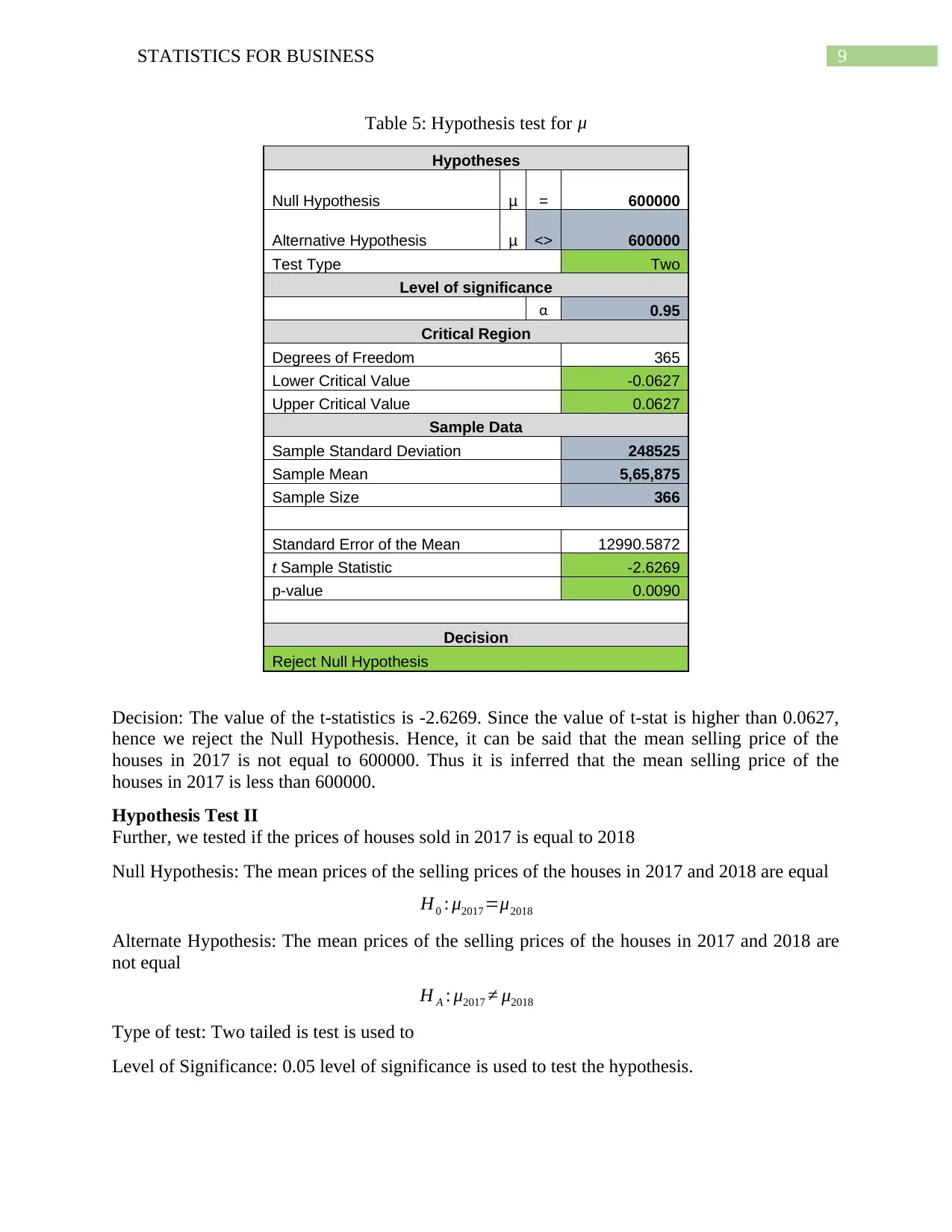
Table 5: Hypothesis test for μ
Hypotheses
Null Hypothesis μ = 600000
Alternative Hypothesis μ <> 600000
Test Type Two
Level of significance
α 0.95
Critical Region
Degrees of Freedom 365
Lower Critical Value -0.0627
Upper Critical Value 0.0627
Sample Data
Sample Standard Deviation 248525
Sample Mean 5,65,875
Sample Size 366
Standard Error of the Mean 12990.5872
t Sample Statistic -2.6269
p-value 0.0090
Decision
Reject Null Hypothesis
Decision: The value of the t-statistics is -2.6269. Since the value of t-stat is higher than 0.0627,
hence we reject the Null Hypothesis. Hence, it can be said that the mean selling price of the
houses in 2017 is not equal to 600000. Thus it is inferred that the mean selling price of the
houses in 2017 is less than 600000.
Hypothesis Test II
Further, we tested if the prices of houses sold in 2017 is equal to 2018
Null Hypothesis: The mean prices of the selling prices of the houses in 2017 and 2018 are equal
H0 : μ2017=μ2018
Alternate Hypothesis: The mean prices of the selling prices of the houses in 2017 and 2018 are
not equal
H A : μ2017 ≠ μ2018
Type of test: Two tailed is test is used to
Level of Significance: 0.05 level of significance is used to test the hypothesis.

10STATISTICS FOR BUSINESS
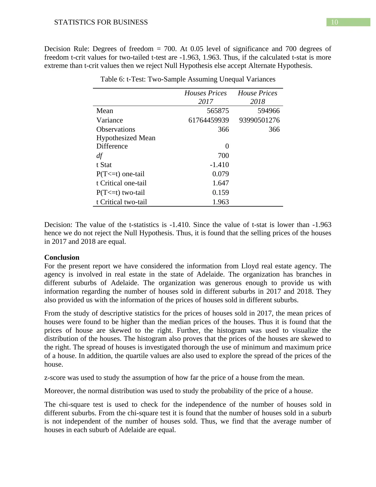
Decision Rule: Degrees of freedom = 700. At 0.05 level of significance and 700 degrees of
freedom t-crit values for two-tailed t-test are -1.963, 1.963. Thus, if the calculated t-stat is more
extreme than t-crit values then we reject Null Hypothesis else accept Alternate Hypothesis.
Table 6: t-Test: Two-Sample Assuming Unequal Variances
Houses Prices
2017
House Prices
2018
Mean 565875 594966
Variance 61764459939 93990501276
Observations 366 366
Hypothesized Mean
Difference 0
df 700
t Stat -1.410
P(T<=t) one-tail 0.079
t Critical one-tail 1.647
P(T<=t) two-tail 0.159
t Critical two-tail 1.963
Decision: The value of the t-statistics is -1.410. Since the value of t-stat is lower than -1.963
hence we do not reject the Null Hypothesis. Thus, it is found that the selling prices of the houses
in 2017 and 2018 are equal.
Conclusion
For the present report we have considered the information from Lloyd real estate agency. The
agency is involved in real estate in the state of Adelaide. The organization has branches in
different suburbs of Adelaide. The organization was generous enough to provide us with
information regarding the number of houses sold in different suburbs in 2017 and 2018. They
also provided us with the information of the prices of houses sold in different suburbs.
From the study of descriptive statistics for the prices of houses sold in 2017, the mean prices of
houses were found to be higher than the median prices of the houses. Thus it is found that the
prices of house are skewed to the right. Further, the histogram was used to visualize the
distribution of the houses. The histogram also proves that the prices of the houses are skewed to
the right. The spread of houses is investigated thorough the use of minimum and maximum price
of a house. In addition, the quartile values are also used to explore the spread of the prices of the
house.
z-score was used to study the assumption of how far the price of a house from the mean.
Moreover, the normal distribution was used to study the probability of the price of a house.
The chi-square test is used to check for the independence of the number of houses sold in
different suburbs. From the chi-square test it is found that the number of houses sold in a suburb
is not independent of the number of houses sold. Thus, we find that the average number of
houses in each suburb of Adelaide are equal.

11STATISTICS FOR BUSINESS
In addition, two hypothesis test is done. In the first hypothesis test a one sample t-test is used.
The one-sample t-test is used to investigate if the price of a house is equivalent to a given price.
The one-sample t-test proves that the mean prices of houses sold in 2017 is less than 600000. In
the second hypothesis test independent sample t-test is used. The independent sample t-test is
used to investigate is the mean price of a house sold in 2017 is different than 2018. In addition,
we find that the mean prices of houses sold in 2017 is equal to the mean prices sold in 2018.