Household Data Analysis: Statistics for Business & Finance Task

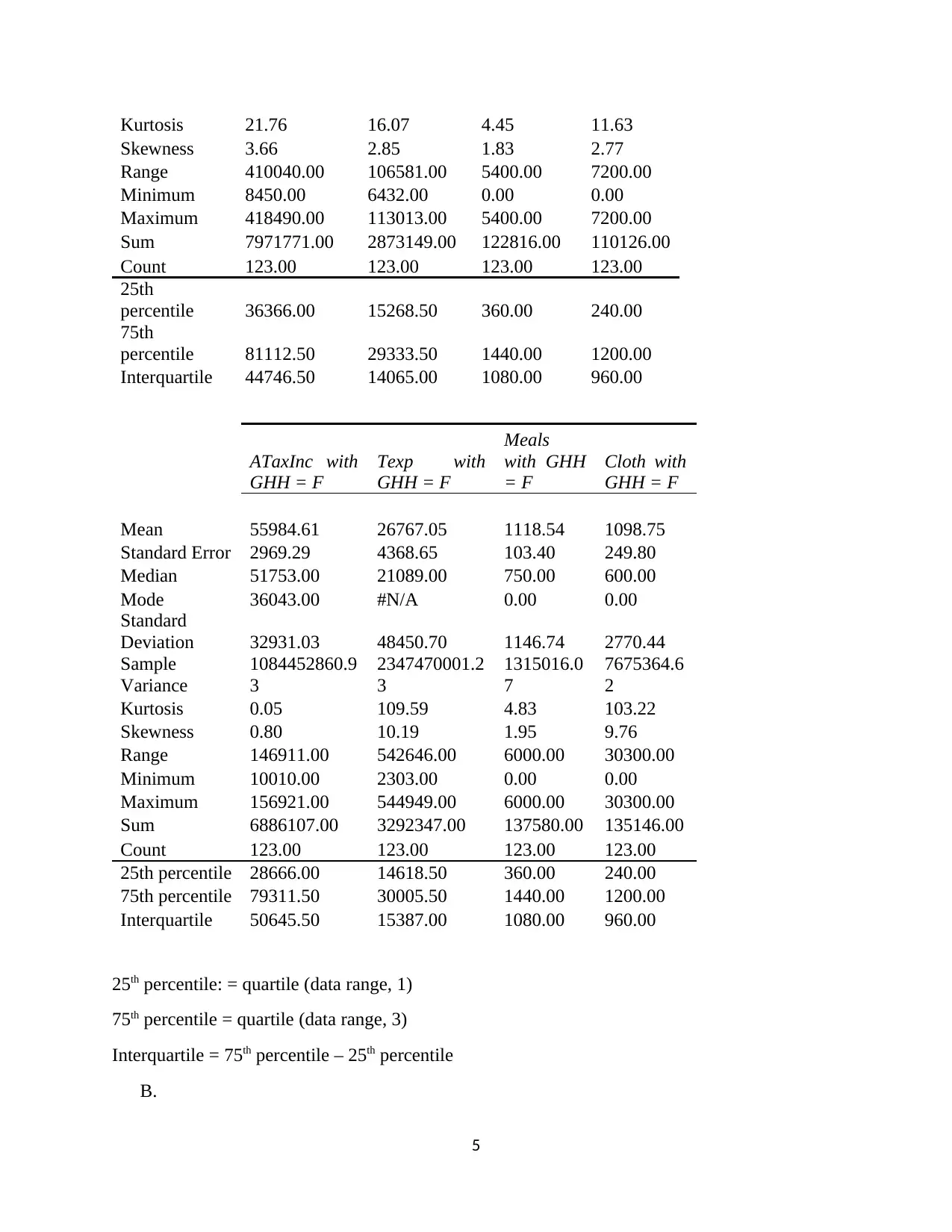
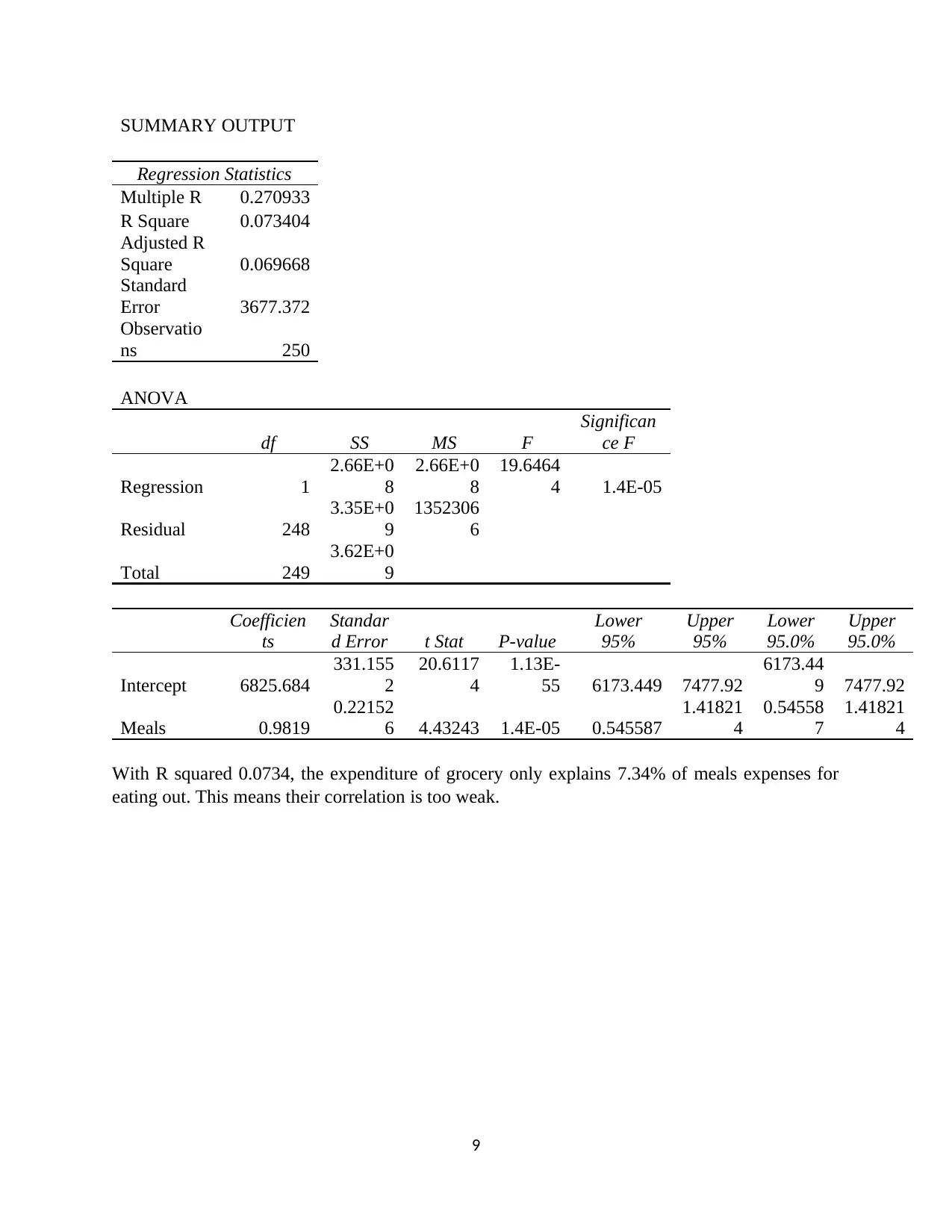
This assignment provides a detailed statistical analysis of household data, examining income, expenditures, and the influence of household head gender. The analysis includes descriptive statistics such as mean, median, mode, standard deviation, skewness, and kurtosis for various financial variables. It explores the differences in income and spending patterns between households headed by males and females, revealing insights into savings behavior and expenditure priorities. Additionally, the assignment investigates the correlation between household size and homeownership, using contingency tables and regression analysis to determine the relationship between grocery expenditure and meals eaten out. The findings indicate weak correlations and highlight the statistical characteristics of the data distributions, including the presence of outliers and skewness. Desklib offers this and many other solved assignments and past papers for students.

Statistics for Business and Finance
Assignment 1 – Examining Household data
Phuc Thang Nguyen
Student number: 20170603
1

Task 1: Preparing data for analysis
Task 2: Describing data
A.
ATaxInc Texp Meals Cloth
Mean AUD 63,409.96 AUD 25,367.54 AUD 1,064.14 AUD 1,007.49
Standard Error AUD 3,145.37 AUD 2,234.51 AUD 66.53 AUD 131.49
Median AUD 54,010.50 AUD 20,847.00 AUD 720.00 AUD 600.00
Mode AUD 36,043.00 AUD 14,998.00 AUD 0.00 AUD 600.00
Standard
Deviation AUD 49,732.66 AUD 35,330.75 AUD 1,051.99 AUD 2,079.07
Sample
Variance
AUD
2,473,337,411.89
AUD
1,248,261,749.31
AUD
1,106,686.53
AUD
4,322,542.23
Kurtosis AUD 20.45 AUD 189.59 AUD 4.89 AUD 159.53
Skewness AUD 3.51 AUD 12.95 AUD 1.92 AUD 11.49
Range AUD 410,040.00 AUD 542,646.00 AUD 6,000.00 AUD 30,300.00
Minimum AUD 8,450.00 AUD 2,303.00 AUD 0.00 AUD 0.00
Maximum AUD 418,490.00 AUD 544,949.00 AUD 6,000.00 AUD 30,300.00
Sum AUD 15,852,489.00 AUD 6,341,886.00
AUD
266,036.00 AUD 251,872.00
Count AUD 250.00 AUD 250.00 AUD 250.00 AUD 250.00
25th percentile AUD 31,565.25 AUD 15,006.75 AUD 360.00 AUD 240.00
75th percentile AUD 80,763.00 AUD 29,503.25 AUD 1,440.00 AUD 1,200.00
Interquartile AUD 49,197.75 AUD 14,496.50 AUD 1,080.00 AUD 960.00
25th percentile: = quartile (data range, 1)
75th percentile = quartile (data range, 3)
Interquartile = 75th percentile – 25th percentile
B.
Location parameter determines the location of a distribution. Location parameter is consisted of
mean, median, and mode. (Thomas, 2015). Mean is the arithmetic average value of a data set.
Median is the midpoint of a data set which half of observations lies above and below. Mode is
the most frequent number in the data set (Michael, 2013).
Spread of a data set is illustrated by standard deviation and variance. Standard deviation is square
root of variance. They measure how far numbers from their means.
Skewness measures how asymmetry of a distribution. (James and Mark, 2008). A normal
distribution has skewness of 0.
2

Kurtosis states how peaked and tail’s mass of a distribution from a normal one. James and Mark
(2008, p.25) states that “the greater the kurtosis of a distribution, the more likely are outliers”.
Kurtosis of a normal distribution equals three.
C.
Mean of “ATaxInc” is the highest at AUD 63,409.96, indicating net average household income
per year at AUD 63,409.96. This figure is higher 2.5-time than total average household
expenditures per year (around AUD 25,367.54). Average annual meals expenditure (AUD
1,064.14) is higher than average annual clothing expenditures (AUD 1,007.49), meaning people
pay more for meals.
Median of “ATaxInc” represents the center of net household income per year in Australia at
AUD 54,010.50. This is much greater than median of “Texp”, which is total household
expenditures yearly. Median of “Meals” and “Cloth” is relatively equally.
Mode of “ATaxInc” is at AUD 36,043.00, indicating many people earns net annual income at
AUD 36,043.00. It is noted that mode of “Meals” is zero, meaning many people did not spend
meals eaten out.
D.
E.
Net household income per year of Australians concentrates on the lower range from AUD35,786
to AUD117,794. As a result, distribution of “ATaxInc” is negatively skewed.
The majority of total household expenses yearly of Australians lies in AUD38,479.4.
3
8450.00
63122.00
117794.00
172466.00
227138.00
281810.00
336482.00
391154.00
0
40
80
Histogram of ATaxInc
Frequency
Bin
Frequency
2303.00
74655.80
147008.60
219361.40
291714.20
364067.00
436419.80
508772.60
0
100
200
Histogram of Texp
Frequency
Bin
Frequency

The majority of meals expenditures of people in Australia ranges from 0 to AUD2,400.
People mainly spent around AUD2,020 on clothing and rarely people bought high-end clothing.
F. Although bin ranges of each variable are difference, the distributions of all variables are
negatively skewed.
Task 3: Describing data conditional on the sex of the household head.
A.
ATaxInc with
GHH = M
Texp with
GHH = M
Meals with
GHH = M
Cloth
with GHH
= M
Mean 64811.15 23358.93 998.50 895.33
Standard
Error 4472.86 1196.09 86.42 93.98
Median 57253.00 20410.00 720.00 600.00
Mode #N/A #N/A 0.00 600.00
Standard
Deviation 49606.41 13265.31 958.48 1042.32
Sample
Variance
2460795623.
96
175968321.
18 918684.10
1086439.9
8
4
0.00
800.00
1600.00
2400.00
3200.00
4000.00
4800.00
5600.00
0
40
80
Histogram of "Meals"
Frequency
Bin
Frequency
0.00
4040.00
8080.00
12120.00
16160.00
20200.00
24240.00
28280.00
0
100
200
Histogram of "Cloth"
Frequency
Bin
Frequency

Kurtosis 21.76 16.07 4.45 11.63
Skewness 3.66 2.85 1.83 2.77
Range 410040.00 106581.00 5400.00 7200.00
Minimum 8450.00 6432.00 0.00 0.00
Maximum 418490.00 113013.00 5400.00 7200.00
Sum 7971771.00 2873149.00 122816.00 110126.00
Count 123.00 123.00 123.00 123.00
25th
percentile 36366.00 15268.50 360.00 240.00
75th
percentile 81112.50 29333.50 1440.00 1200.00
Interquartile 44746.50 14065.00 1080.00 960.00
ATaxInc with
GHH = F
Texp with
GHH = F
Meals
with GHH
= F
Cloth with
GHH = F
Mean 55984.61 26767.05 1118.54 1098.75
Standard Error 2969.29 4368.65 103.40 249.80
Median 51753.00 21089.00 750.00 600.00
Mode 36043.00 #N/A 0.00 0.00
Standard
Deviation 32931.03 48450.70 1146.74 2770.44
Sample
Variance
1084452860.9
3
2347470001.2
3
1315016.0
7
7675364.6
2
Kurtosis 0.05 109.59 4.83 103.22
Skewness 0.80 10.19 1.95 9.76
Range 146911.00 542646.00 6000.00 30300.00
Minimum 10010.00 2303.00 0.00 0.00
Maximum 156921.00 544949.00 6000.00 30300.00
Sum 6886107.00 3292347.00 137580.00 135146.00
Count 123.00 123.00 123.00 123.00
25th percentile 28666.00 14618.50 360.00 240.00
75th percentile 79311.50 30005.50 1440.00 1200.00
Interquartile 50645.50 15387.00 1080.00 960.00
25th percentile: = quartile (data range, 1)
75th percentile = quartile (data range, 3)
Interquartile = 75th percentile – 25th percentile
B.
5

Location parameter determines the location of a distribution. Location parameter is consisted of
mean, median, and mode. (Thomas, 2015). Mean is the arithmetic average value of a data set.
Median is the midpoint of a data set which half of observations lies above and below. Mode is
the most frequent number in the data set (Michael, 2013).
Spread of a data set is illustrated by standard deviation and variance. Standard deviation is square
root of variance. They measure how far numbers from their means.
Skewness measures how asymmetry of a distribution. (James and Mark, 2008). A normal
distribution has skewness of 0.
Kurtosis states how peaked and tail’s mass of a distribution from a normal one. James and Mark
(2008, p.25) states that “the greater the kurtosis of a distribution, the more likely are outliers”.
Kurtosis of a normal distribution equals three.
C.
Interestingly, on average, the household head of male have earned more than that of female but
the household head of female spent more than (in terms of “Texp”, “Meals” and “Cloth”).
Median of “Cloth” between two genders are equal, while median of “meals” expenses is quite
the same.
According to mode, the majority of meals expenditure in eating out for both types of household
head is zero, meaning primarily people prefer home-cooked meals.
Skewness of all variables by both genders is positive, which is greater than one.
Only kurtosis of “ATaxInc” with gender household head of female is less than three, the rest is
higher than three. This means the distribution of “ATaxInc” with female household head is less
peaked than a normal distribution and the rest is more peaked (or flatter).
D.
Household head of male has earned AUD64,811.15 net household income per year,
approximately 2.8-time than average total expenditure per year. Mean of “meals” is higher than
that of “cloth” as male as household head but not much (AUD998.50 and AUD895.30
respectively).
Following the same direction as mean, median of “ATaxInc” is much higher than that of “Texp”,
meaning the male are saving significantly.
Standard deviation of variables for male household head is significant. The considerable standard
deviation implies scattered number in the data set.
The kurtosis of “ATaxInc” is extremely high (at 21.76), implying there are many outliners in its
data set. The kurtosis of “Texp” is also high (at 16.07), which can be examined by box-whisker
plot.
E.
6

On average, a household with head of female earns AUD55,984.61 and spends AUD26,767.05.
The average expenses for meals and clothing account for two fifths of average income.
Standard deviation of all variables for female household head is remarkable, indicating no
concentration of numbers from their means.
“ATaxInc” with gender household head of female kurtosis less than 3, suggesting less peaked
and light-tailed distribution than a normal distribution, and lack of outliers. At the same time,
kurtosis of “Texp” and “Cloth” are highly significantly (in turn 109.59 and 103.22), which
raising a question on outliers in the data set.
While “ATaxInc” of female household head is close to a normal distribution, the remaining
variables are positively skewed which implies large positive outliers pulls the mean upward.
Task 4: Searching for correlation in data
A. First, contingency table is created by using COUNTIFS formula
Own house
Total0 1
No of people in a
household
1 17 26 43
2 0 0 0
3 7 7 14
4 0 0 0
5 2 2 4
6 0 0 0
7 1 1 2
8 1 1 2
Total 28 37 65
Then, I calculate contingency table under percentage
7

Own house
Total0 1
No of people in a
household
1 26.15% 40.00% 66.15%
2 0.00% 0.00% 0.00%
3 10.77% 10.77% 21.54%
4 0.00% 0.00% 0.00%
5 3.08% 3.08% 6.15%
6 0.00% 0.00% 0.00%
7 1.54% 1.54% 3.08%
8 1.54% 1.54% 3.08%
Total 43.08% 56.92%
100.00
%
From the above table, probability of a 5-person household which does not own a house is 3.08%.
B.
From the table, a larger household is not likely to own a house. As the probability a household
with one person owning a house is 66.15% and the probability a household of 3 people owning a
house is 21.54%. Such figures are significantly higher than probability of household of 7 and 8
people who can own a house, at 3.08%.
C.
8
0 1000 2000 3000 4000 5000 6000 7000
0
5000
10000
15000
20000
25000
30000
f(x) = 0.981900480007965 x + 6825.6844956024
R² = 0.0734044340414016
Single linear regression between grocery and meals
Meals expenditure (AUD)
Grocery expenditure (AUD)

SUMMARY OUTPUT
Regression Statistics
Multiple R 0.270933
R Square 0.073404
Adjusted R
Square 0.069668
Standard
Error 3677.372
Observatio
ns 250
ANOVA
df SS MS F
Significan
ce F
Regression 1
2.66E+0
8
2.66E+0
8
19.6464
4 1.4E-05
Residual 248
3.35E+0
9
1352306
6
Total 249
3.62E+0
9
Coefficien
ts
Standar
d Error t Stat P-value
Lower
95%
Upper
95%
Lower
95.0%
Upper
95.0%
Intercept 6825.684
331.155
2
20.6117
4
1.13E-
55 6173.449 7477.92
6173.44
9 7477.92
Meals 0.9819
0.22152
6 4.43243 1.4E-05 0.545587
1.41821
4
0.54558
7
1.41821
4
With R squared 0.0734, the expenditure of grocery only explains 7.34% of meals expenses for
eating out. This means their correlation is too weak.
9

Reference
Stock, J. and W. Watson, M. (2019). Introduction to Econometrics, Third edition update.
3rd ed. Boston: Pearson, pp.23-25.
Haslwanter, T. (2016). An Introduction to Statistics with Python with Applications in the
Life Sciences. 1st ed. Switzerland: Springer International Publishing, p.96.
B. Miller, M. (2019). Mathematics & Statistics for Financial Risk Management. 2nd ed.
New Jersey: John Wiley & Sons, Inc., p.30.
10