Statistics for Business Decisions

This solved assignment explores statistical concepts and techniques applied to business decisions. It analyzes Australian export data, constructs frequency distributions, plots histograms and ogive charts, calculates descriptive statistics, and investigates the relationship between final consumption expenditure and retail turnover per capita using correlation and regression analysis.

Statistics for Business Decisions

Table of Contents
INTRODUCTION...........................................................................................................................4
QUESTION 1..................................................................................................................................4
a. Using an appropriate graphical technique to compare the value of Australian exports..........4
b. Using an appropriate graphical technique to compare the percentage value of Australian
exports (in %)..............................................................................................................................5
c. Commenting on observation....................................................................................................6
QUESTION 2..................................................................................................................................7
a. Constructing a frequency and relative frequency distribution for the data set given..............7
b. Construct a cumulative frequency and relative distribution....................................................7
c. Plotting a relative frequency histogram for the data................................................................8
d. Ogive chart...............................................................................................................................8
e. Stating proportion of the grades which is less than 60............................................................8
f. Stating proportion of the grades which is more than 70...........................................................9
QUESTION 3..................................................................................................................................9
a. Using an appropriate graphical descriptive measure for describing two variables..................9
b. Investigating the relationship between final consumption expenditure and retail turnover per
capita..........................................................................................................................................10
c. Descriptive statistics..............................................................................................................10
d. Calculating coefficient of correlation (r) between two concerned variables.........................12
f..................................................................................................................................................13
g.................................................................................................................................................13
h.................................................................................................................................................15
CONCLUSION..............................................................................................................................15
REFERENCES..............................................................................................................................16

INTRODUCTION
In the current times, business managers lay high level of emphasis on undertaking
statistical tools and techniques with the motive to develop appropriate framework for decision
making. Moreover, statistical tools helps in exhibiting, analysing and evaluating large data set in
a highly structured format (Silverman, 2018). The present report is based on different case
situations which will provide deeper insight how graphical presentation helps in understanding
data set effectually. Besides this, report will also develop understanding about the aspects in
relation to descriptive statistics, ogive chart etc. It also depicts the manner in which regression
tool helps in assessing relationship between two concerned variables.
QUESTION 1
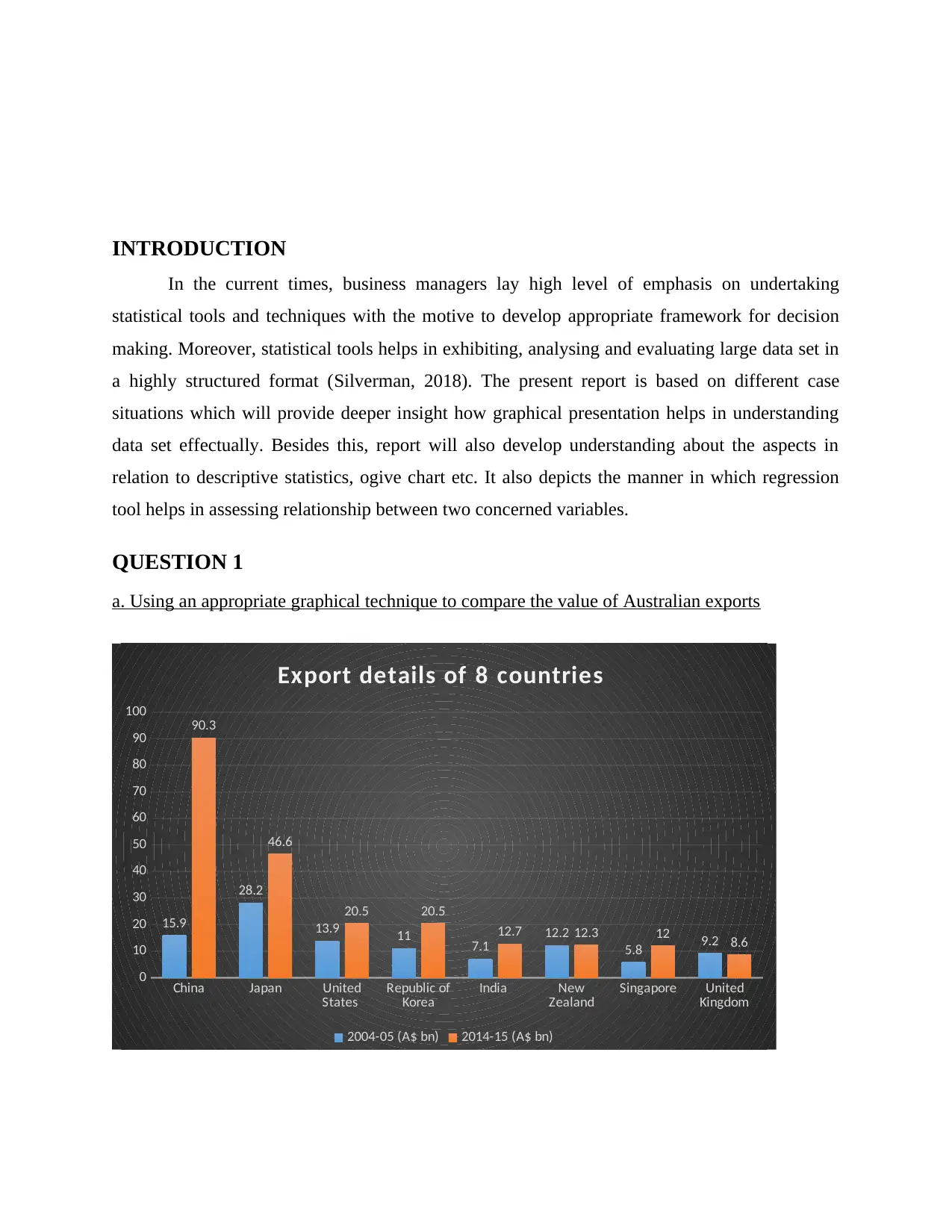
a. Using an appropriate graphical technique to compare the value of Australian exports
China Japan United
States Republic of
Korea India New
Zealand Singapore United
Kingdom
0
10
20
30
40
50
60
70
80
90
100
15.9
28.2
13.9 11 7.1 12.2
5.8 9.2
90.3
46.6
20.5 20.5
12.7 12.3 12 8.6
Export details of 8 countries
2004-05 (A$ bn) 2014-15 (A$ bn)

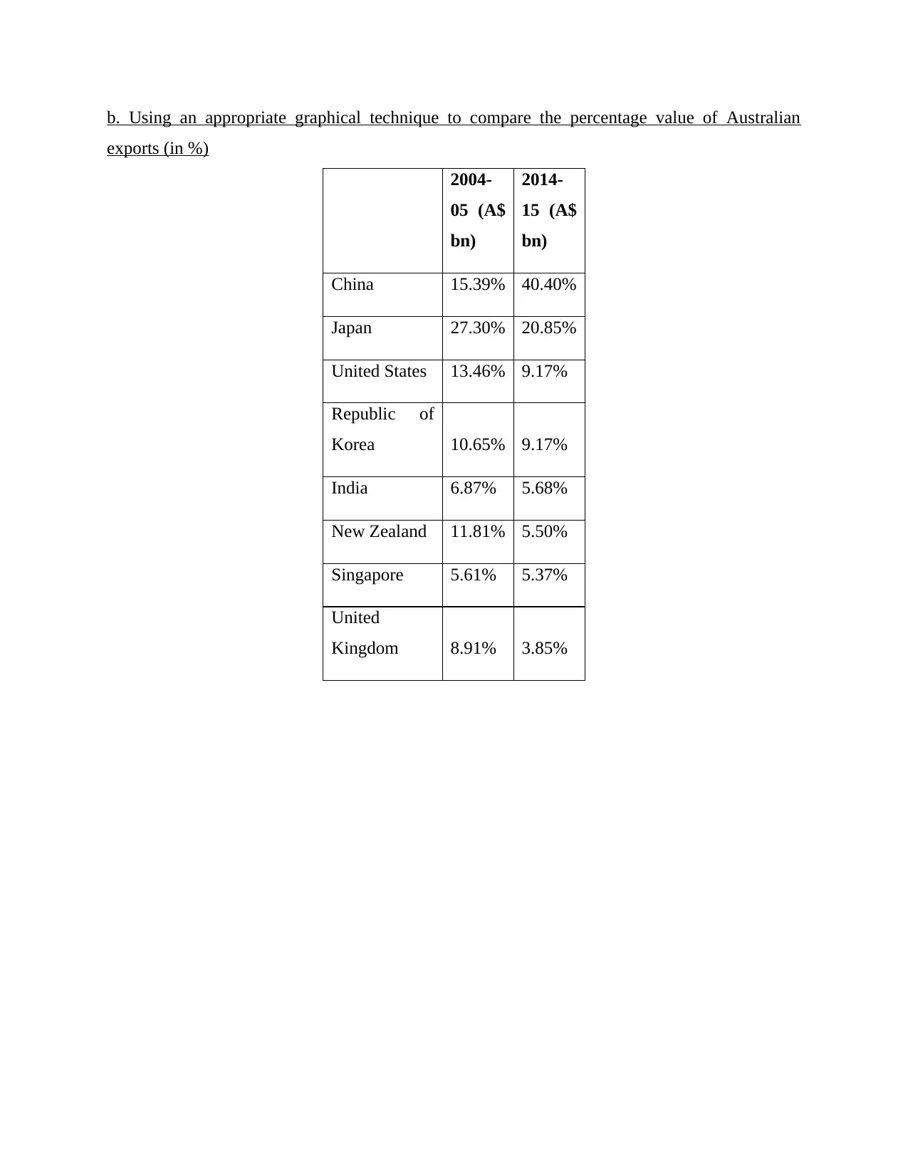
b. Using an appropriate graphical technique to compare the percentage value of Australian
exports (in %)
2004-
05 (A$
bn)
2014-
15 (A$
bn)
China 15.39% 40.40%
Japan 27.30% 20.85%
United States 13.46% 9.17%
Republic of
Korea 10.65% 9.17%
India 6.87% 5.68%
New Zealand 11.81% 5.50%
Singapore 5.61% 5.37%
United
Kingdom 8.91% 3.85%

China Japan United States Republic of
Korea India New Zealand Singapore United
Kingdom
0.00%
5.00%
10.00%
15.00%
20.00%
25.00%
30.00%
35.00%
40.00%
45.00%
15.39%
27.30%
13.46%
10.65%
6.87%
11.81%
5.61%
8.91%
40.40%
20.85%
9.17% 9.17%
5.68% 5.50% 5.37% 3.85%
Export details of 8 countries
(in %)
2004-05 (A$ bn) 2014-15 (A$ bn)
c. Commenting on observation
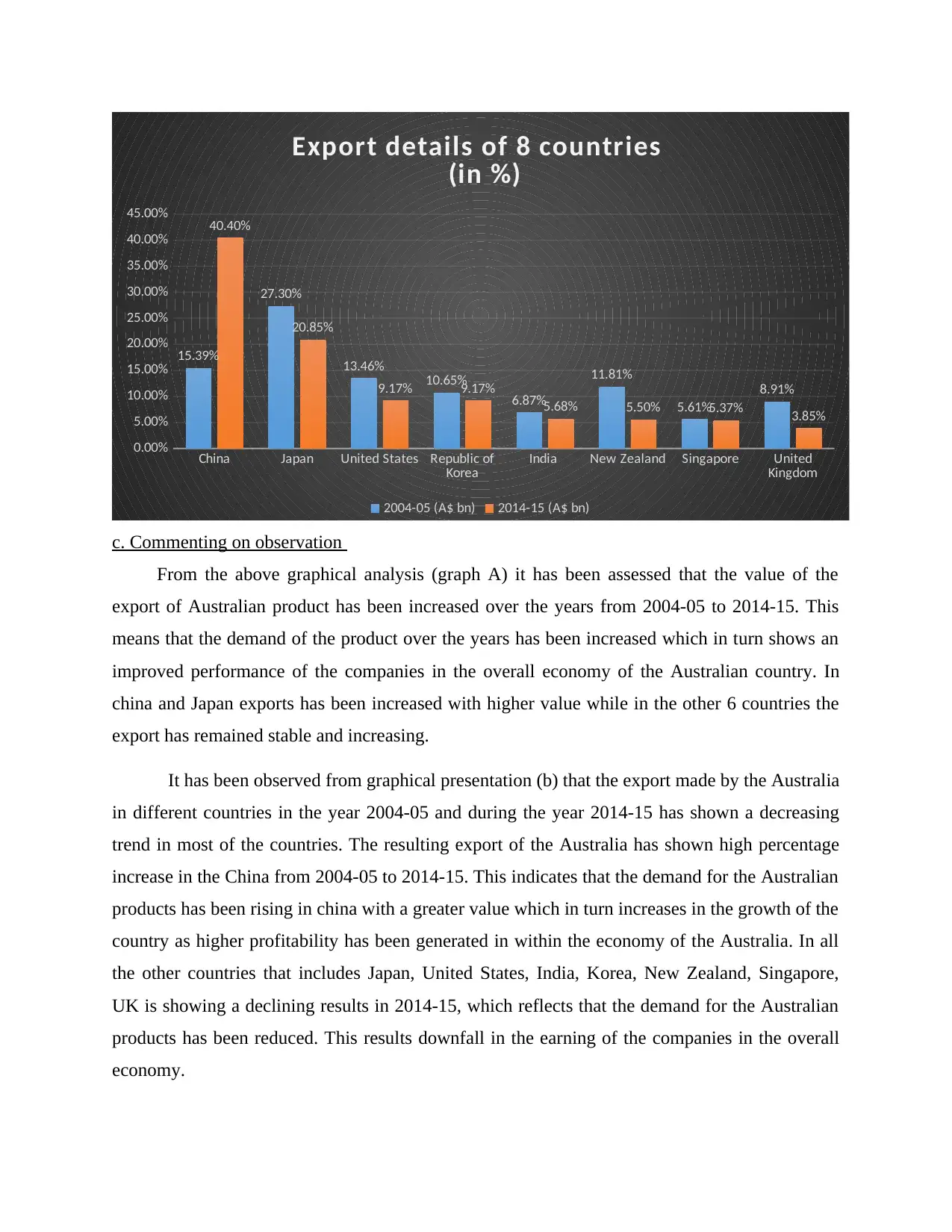
From the above graphical analysis (graph A) it has been assessed that the value of the
export of Australian product has been increased over the years from 2004-05 to 2014-15. This
means that the demand of the product over the years has been increased which in turn shows an
improved performance of the companies in the overall economy of the Australian country. In
china and Japan exports has been increased with higher value while in the other 6 countries the
export has remained stable and increasing.
It has been observed from graphical presentation (b) that the export made by the Australia
in different countries in the year 2004-05 and during the year 2014-15 has shown a decreasing
trend in most of the countries. The resulting export of the Australia has shown high percentage
increase in the China from 2004-05 to 2014-15. This indicates that the demand for the Australian
products has been rising in china with a greater value which in turn increases in the growth of the
country as higher profitability has been generated in within the economy of the Australia. In all
the other countries that includes Japan, United States, India, Korea, New Zealand, Singapore,
UK is showing a declining results in 2014-15, which reflects that the demand for the Australian
products has been reduced. This results downfall in the earning of the companies in the overall
economy.

QUESTION 2
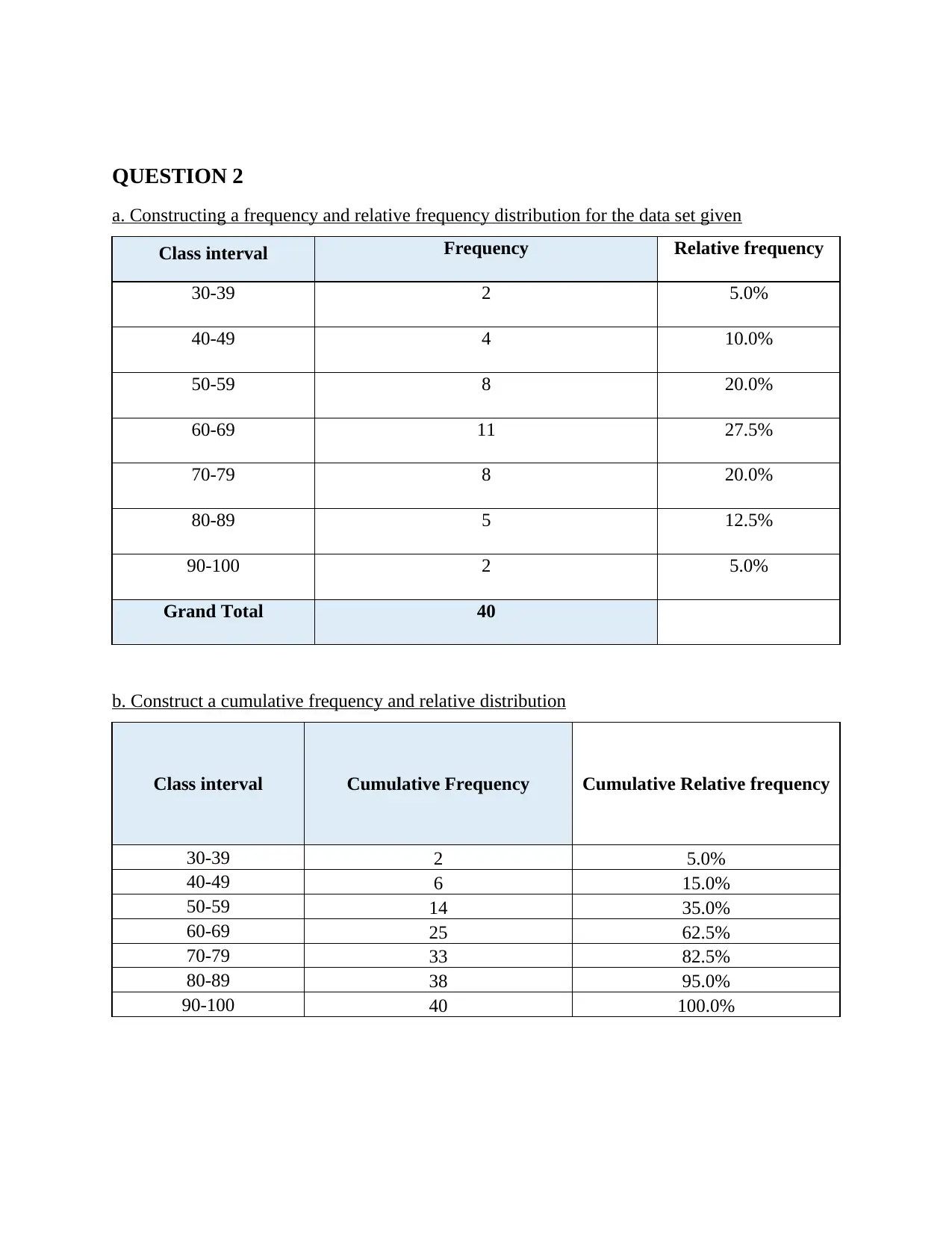
a. Constructing a frequency and relative frequency distribution for the data set given
Class interval Frequency Relative frequency
30-39 2 5.0%
40-49 4 10.0%
50-59 8 20.0%
60-69 11 27.5%
70-79 8 20.0%
80-89 5 12.5%
90-100 2 5.0%
Grand Total 40
b. Construct a cumulative frequency and relative distribution
Class interval Cumulative Frequency Cumulative Relative frequency
30-39 2 5.0%
40-49 6 15.0%
50-59 14 35.0%
60-69 25 62.5%
70-79 33 82.5%
80-89 38 95.0%
90-100 40 100.0%

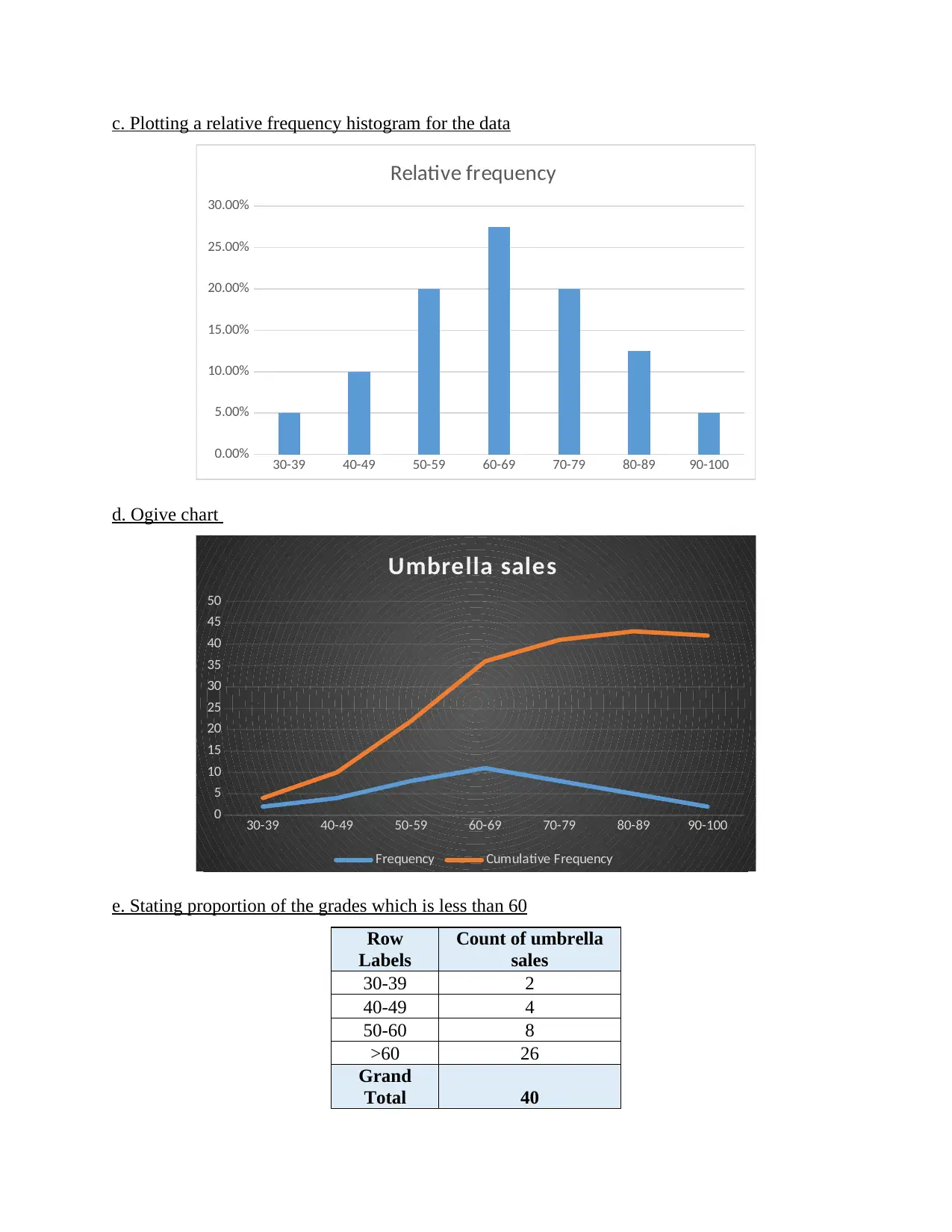
c. Plotting a relative frequency histogram for the data
30-39 40-49 50-59 60-69 70-79 80-89 90-100
0.00%
5.00%
10.00%
15.00%
20.00%
25.00%
30.00%
Relative frequency
d. Ogive chart
30-39 40-49 50-59 60-69 70-79 80-89 90-100
0
5
10
15
20
25
30
35
40
45
50
Umbrella sales
Frequency Cumulative Frequency
e. Stating proportion of the grades which is less than 60
Row
Labels
Count of umbrella
sales
30-39 2
40-49 4
50-60 8
>60 26
Grand
Total 40

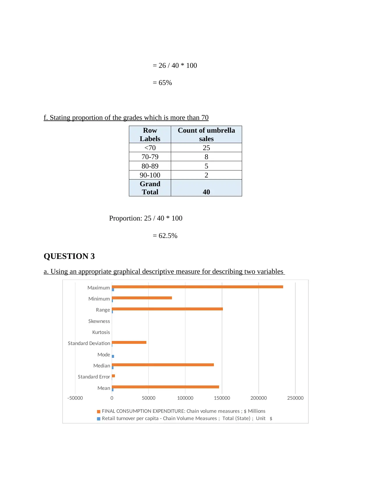
= 26 / 40 * 100
= 65%
f. Stating proportion of the grades which is more than 70
Row
Labels
Count of umbrella
sales
<70 25
70-79 8
80-89 5
90-100 2
Grand
Total 40
Proportion: 25 / 40 * 100
= 62.5%
QUESTION 3
a. Using an appropriate graphical descriptive measure for describing two variables
Mean
Standard Error
Median
Mode
Standard Deviation
Kurtosis
Skewness
Range
Minimum
Maximum
-50000 0 50000 100000 150000 200000 250000
FINAL CONSUMPTION EXPENDITURE: Chain volume measures ; $ Millions
Retail turnover per capita - Chain Volume Measures ; Total (State) ; Unit $

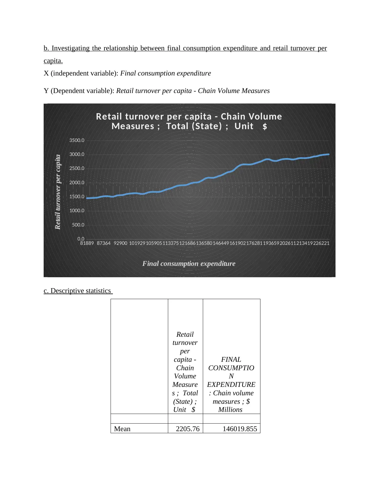
b. Investigating the relationship between final consumption expenditure and retail turnover per
capita.
X (independent variable): Final consumption expenditure
Y (Dependent variable): Retail turnover per capita - Chain Volume Measures
81889 87364 92900 101929105905113375121686136580146449161902176281193659202611213419226221
0.0
500.0
1000.0
1500.0
2000.0
2500.0
3000.0
3500.0
Retail turnover per capita - Chain Volume
Measures ; Total (State) ; Unit $
Final consumption expenditure
Retail turnover per capita
c. Descriptive statistics
Retail
turnover
per
capita -
Chain
Volume
Measure
s ; Total
(State) ;
Unit $
FINAL
CONSUMPTIO
N
EXPENDITURE
: Chain volume
measures ; $
Millions
Mean 2205.76 146019.855

Standard Error 47.4591 4098.05042
Median 2180.2 139137
Mode 2852.8 #N/A
Standard
Deviation 543.194 46904.331
Kurtosis -1.612 -1.2960945
Skewness 0.07466 0.30683061
Range 1558.7 151259
Minimum 1455.9 81889
Maximum 3014.6 233148
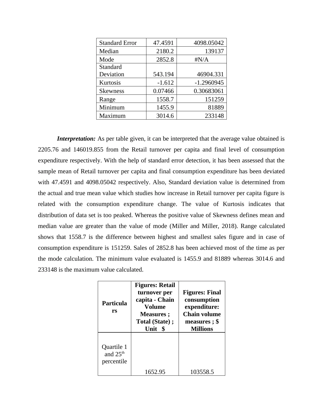
Interpretation: As per table given, it can be interpreted that the average value obtained is
2205.76 and 146019.855 from the Retail turnover per capita and final level of consumption
expenditure respectively. With the help of standard error detection, it has been assessed that the
sample mean of Retail turnover per capita and final consumption expenditure has been deviated
with 47.4591 and 4098.05042 respectively. Also, Standard deviation value is determined from
the actual and true mean value which studies how increase in Retail turnover per capita figure is
related with the consumption expenditure change. The value of Kurtosis indicates that
distribution of data set is too peaked. Whereas the positive value of Skewness defines mean and
median value are greater than the value of mode (Miller and Miller, 2018). Range calculated
shows that 1558.7 is the difference between highest and smallest sales figure and in case of
consumption expenditure is 151259. Sales of 2852.8 has been achieved most of the time as per
the mode calculation. The minimum value evaluated is 1455.9 and 81889 whereas 3014.6 and
233148 is the maximum value calculated.
Particula
rs
Figures: Retail
turnover per
capita - Chain
Volume
Measures ;
Total (State) ;
Unit $
Figures: Final
consumption
expenditure:
Chain volume
measures ; $
Millions
Quartile 1
and 25th
percentile
1652.95 103558.5

Quartile 2
and 50th
percentile
2180.2 139137
Quartile 3
and 75h
percentile
2793.4 192800.5
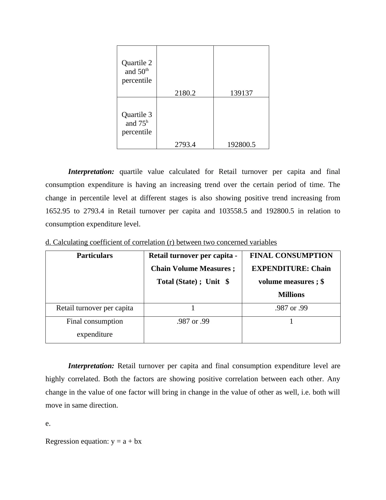
Interpretation: quartile value calculated for Retail turnover per capita and final
consumption expenditure is having an increasing trend over the certain period of time. The
change in percentile level at different stages is also showing positive trend increasing from
1652.95 to 2793.4 in Retail turnover per capita and 103558.5 and 192800.5 in relation to
consumption expenditure level.
d. Calculating coefficient of correlation (r) between two concerned variables
Particulars Retail turnover per capita -
Chain Volume Measures ;
Total (State) ; Unit $
FINAL CONSUMPTION
EXPENDITURE: Chain
volume measures ; $
Millions
Retail turnover per capita 1 .987 or .99
Final consumption
expenditure
.987 or .99 1
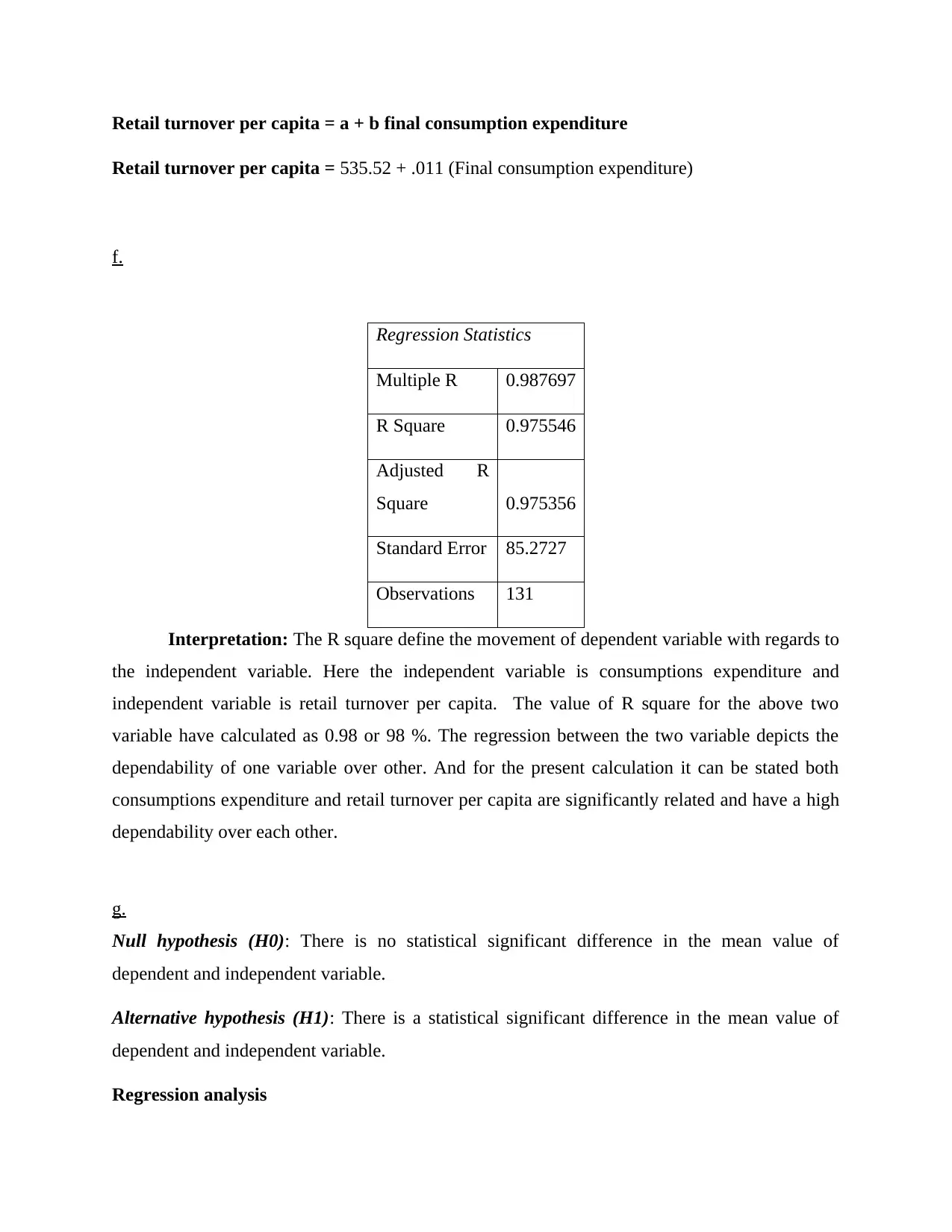
Interpretation: Retail turnover per capita and final consumption expenditure level are
highly correlated. Both the factors are showing positive correlation between each other. Any
change in the value of one factor will bring in change in the value of other as well, i.e. both will
move in same direction.
e.
Regression equation: y = a + bx

Retail turnover per capita = a + b final consumption expenditure
Retail turnover per capita = 535.52 + .011 (Final consumption expenditure)
f.
Regression Statistics
Multiple R 0.987697
R Square 0.975546
Adjusted R
Square 0.975356
Standard Error 85.2727
Observations 131
Interpretation: The R square define the movement of dependent variable with regards to
the independent variable. Here the independent variable is consumptions expenditure and
independent variable is retail turnover per capita. The value of R square for the above two
variable have calculated as 0.98 or 98 %. The regression between the two variable depicts the
dependability of one variable over other. And for the present calculation it can be stated both
consumptions expenditure and retail turnover per capita are significantly related and have a high
dependability over each other.
g.
Null hypothesis (H0): There is no statistical significant difference in the mean value of
dependent and independent variable.
Alternative hypothesis (H1): There is a statistical significant difference in the mean value of
dependent and independent variable.
Regression analysis

ANOV
A
df SS MS F
Significan
ce F
Regressi
on 1
374197
33
374197
33
5146.1
29 7.9E-106
Residual 129
938014.
9
7271.43
3
Total 130
383577
47
Coef
ficie
nts
Stand
ard
Error
t
Stat
P-
val
ue
Low
er
95%
Upp
er
95%
Lowe
r
95.0
%
Uppe
r
95.0
%
Intercept
535.
5266
24.44
588
21.
906
62
2.6
7E-
45
487.
1599
583.
8934
487.1
599
583.8
934
FINAL CONSUMPTION
EXPENDITURE: Chain volume
measures ; $ Millions
0.01
1438
0.000
159
71.
736
52
7.9
E-
106
0.01
1123
0.01
1754
0.011
123
0.011
754
Interpretation:
The value of p for this calculation is less than significant level of 5% that is 0.05 this means the
alternative hypothesis is accepted here (Magnus and Neudecker, 2019). This can be stated that
there is a statistical significant difference in the mean value of final consumption expenditure and
retail turnover per capita.

h.
Regression Statistics
Standard Error 85.2727
Interpretation: The value of standard error of the estimate is 85.27. This is the square
root of the residual mean square which represent the accuracy with with samples represent the
population. In the calculation the standard error of estimate have came at 85.27 which means the
accuracy level of sample collection is very high.
CONCLUSION
By summing up this report, it has been concluded that, in the accounting year 2014-15,
export level of China was too higher in comparison to other countries. Besides this, it can be
inferred that in against to Australia, contribution of China and Japan is higher with reference to
export level. Along with this, it has been articulated that retail turnover (per capita) is highly
associated with final consumption expenditure level. Hence, statistically both the variables have
significant impact on each other.

REFERENCES
Books and Journals
Magnus, J. R. and Neudecker, H., 2019. Matrix differential calculus with applications in
statistics and econometrics. Wiley.
Miller, J. and Miller, J. C., 2018. Statistics and chemometrics for analytical chemistry. Pearson
education.
Silverman, B. W., 2018. Density estimation for statistics and data analysis. Routledge.