Holmes Institute HI6007 Statistics for Business Decisions
VerifiedAdded on 2023/06/07
|12
|1603
|290
Homework Assignment
AI Summary
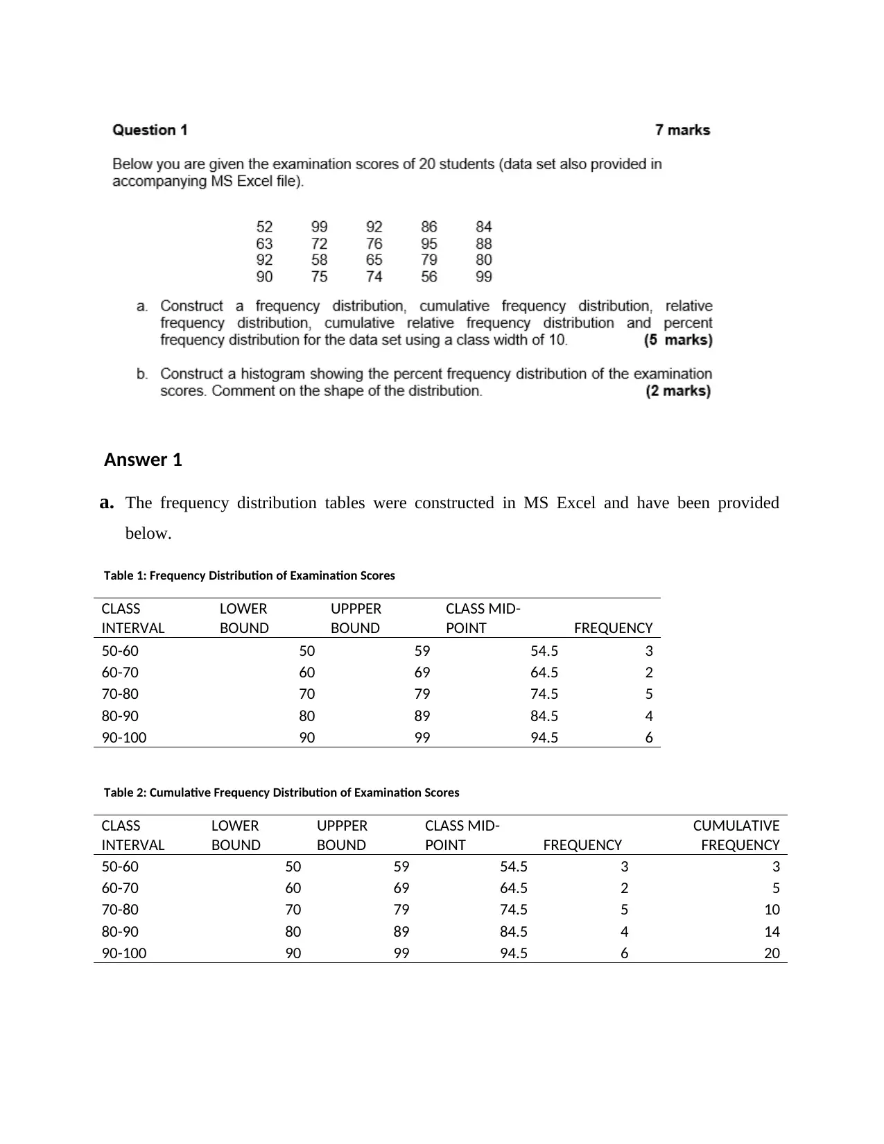
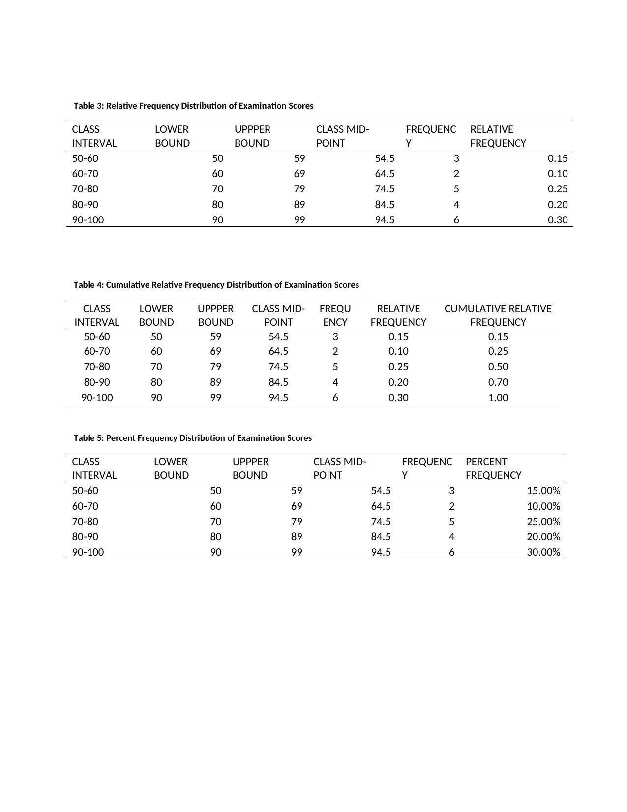
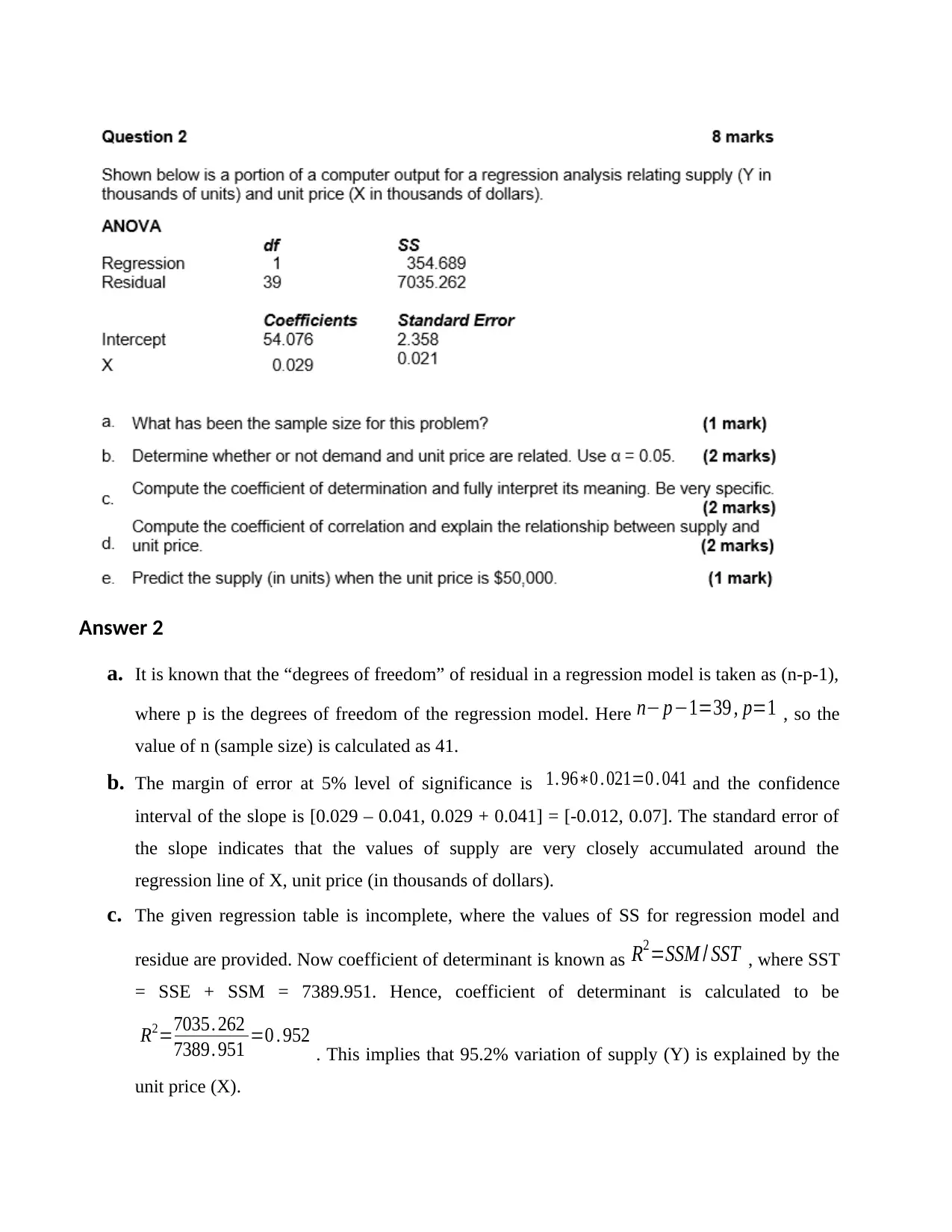
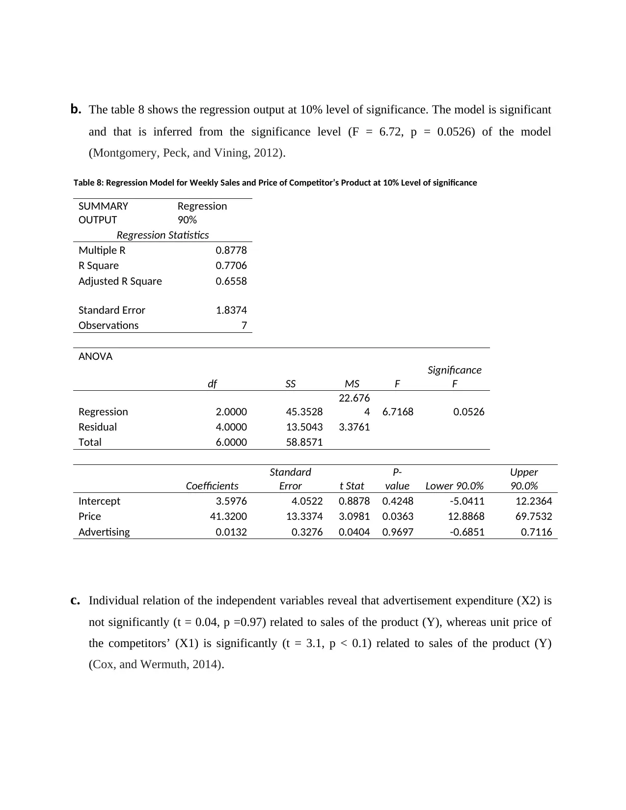
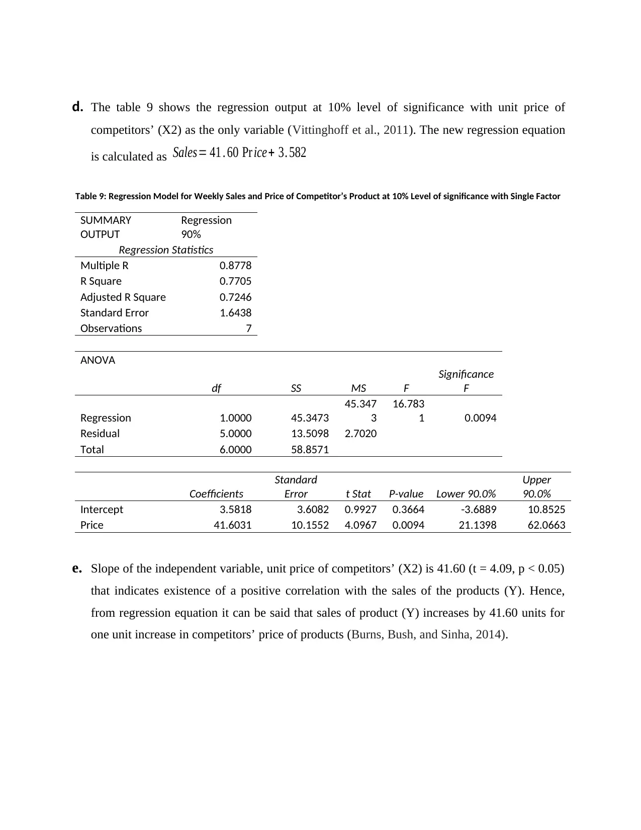
This assignment solution covers key statistical concepts for business decisions, including frequency distributions, regression analysis, and ANOVA. It addresses questions related to examination score analysis, regression model interpretation, and hypothesis testing for comparing different programs within a corporation. The solution includes detailed tables generated in MS Excel, interpretations of statistical outputs, and recommendations based on the analysis. Topics such as cumulative frequency, relative frequency, percentage distribution, correlation coefficients, and significance levels are thoroughly explored. The regression analysis focuses on the relationship between supply and unit price, as well as the impact of competitor pricing on sales. Desklib provides comprehensive resources, including solved assignments and past papers, to support students in mastering these statistical techniques.

1 out of 12
Related Documents


Your All-in-One AI-Powered Toolkit for Academic Success.
+13062052269
info@desklib.com
Available 24*7 on WhatsApp / Email
![[object Object]](/_next/static/media/star-bottom.7253800d.svg)
Copyright © 2020–2025 A2Z Services. All Rights Reserved. Developed and managed by ZUCOL.