Statistics for Business Decisions - PDF

Running Head: STATISTICS FOR BUSINESS DECISIONS
Statistics for business decisions
Name of the Student
Name of the University
Author Note

1STATISTICS FOR BUSINESS DECISIONS
Table of Contents
ANSWER 1.....................................................................................................................................2
ANSWER 2.....................................................................................................................................5
ANSWER 3.....................................................................................................................................7
ANSWER 4...................................................................................................................................10
ANSWER 5...................................................................................................................................13

2STATISTICS FOR BUSINESS DECISIONS
ANSWER 1
Part a
The frequency table can be represented as:
Class Interval Frequency Relative Frequency
Percentage
Frequency
Distribution
150 3 0.06 6.0%
200 15 0.30 30.0%
250 14 0.28 28.0%
300 6 0.12 12.0%
350 4 0.08 8.0%
400 3 0.06 6.0%
450 3 0.06 6.0%
500 2 0.04 4.0%
Part b
150 200 250 300 350 400 450 500
0.0%
5.0%
10.0%
15.0%
20.0%
25.0%
30.0%
35.0%
Percentage Frequency Distribution of Order
Value
Frequency (Order Value)
Percentage of Occurence
Figure 1: Percentage Frequency Distribution of Order Value
From the above histogram it is found that the order values are skewed to the right. Hence
it can be said that the mean order value is greater than the median order value.

3STATISTICS FOR BUSINESS DECISIONS
Part c
Since the histogram is skewed right hence the mean order value is greater than the
median order value.
Thus the median of the order value would be a better measure of the data set. The median
value of the order would represent the value below and above which 50% of the orders are.
ANSWER 2
Anova
df SS MS F Significance F
Regressio
n 1 5048.818 5048.818 74.137 0.000
Residual 46 3132.661 68.101
Total 47 8181.479
Part a
At 0.05 level of significance there is statistically significant relation between demand and unit
price, p-value < 0.000.
Part b
The coefficient of determination ¿ SSM
SST = 5048.818
8181.479 =0.617
Thus, 61.7% of the variability in demand can be predicted from Unit price.
Part c
The coefficient of correlation ¿ √ 0.617=0.786
From the value of coefficient of correlation, it can be said that there is a very strong
correlation between demand and unit price.

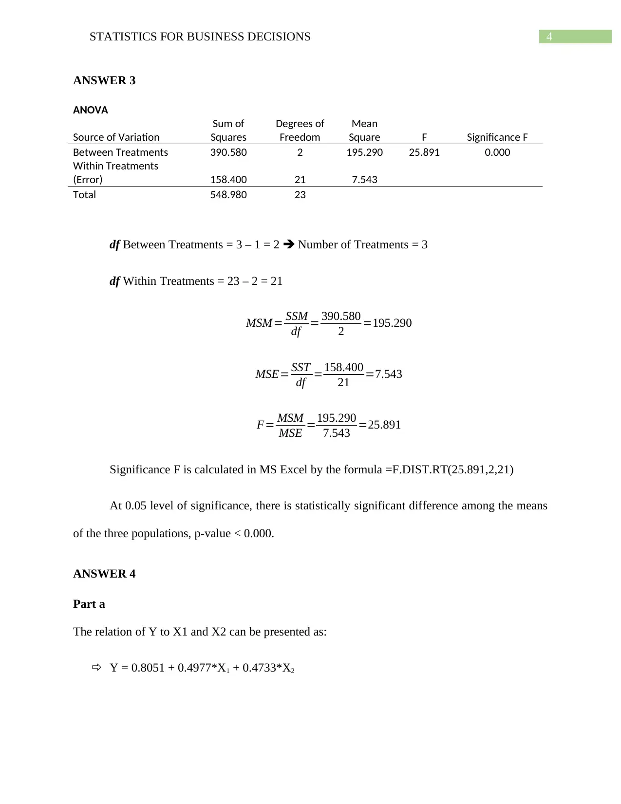
4STATISTICS FOR BUSINESS DECISIONS
ANSWER 3
ANOVA
Source of Variation
Sum of
Squares
Degrees of
Freedom
Mean
Square F Significance F
Between Treatments 390.580 2 195.290 25.891 0.000
Within Treatments
(Error) 158.400 21 7.543
Total 548.980 23
df Between Treatments = 3 – 1 = 2  Number of Treatments = 3
df Within Treatments = 23 – 2 = 21
MSM= SSM
df = 390.580
2 =195.290
MSE= SST
df =158.400
21 =7.543
F= MSM
MSE =195.290
7.543 =25.891
Significance F is calculated in MS Excel by the formula =F.DIST.RT(25.891,2,21)
At 0.05 level of significance, there is statistically significant difference among the means
of the three populations, p-value < 0.000.
ANSWER 4
Part a
The relation of Y to X1 and X2 can be presented as:
 Y = 0.8051 + 0.4977*X1 + 0.4733*X2

5STATISTICS FOR BUSINESS DECISIONS
Part b
ANOVA
df SS MS F Significance F
Regression 1 40.700 40.700 480.709 0.000
Residual 12 1.016 0.085
13 41.716
From the above calculations, it is found that there is statistically significant relation
between the independent and dependent variables, p-value < 0.000 at 0.05 level of significance.
Part c
Coefficients Standard Error t stat
Intercept 0.8051
X1 0.4977 0.4617 1.078
X2 0.4733 0.0387 12.230
t-stat for X1 ¿ 0.4977
0.4617 =1.080
t-stat for X2 = 0.4733
0.0387 =12.230
The tabulated t-value at 0.05 level of significance and 13 degrees of freedom is 2.16
Since, the t-stat is less than the tabulated value for Price (1.078 < 2.16), hence, the value
of Price (X1) is significantly not different from zero.
Since, the t-stat is more than the tabulated value for Advertising spots (12.230 > 2.16)
hence the value of Advertising Spots (X2) is significantly different from zero.

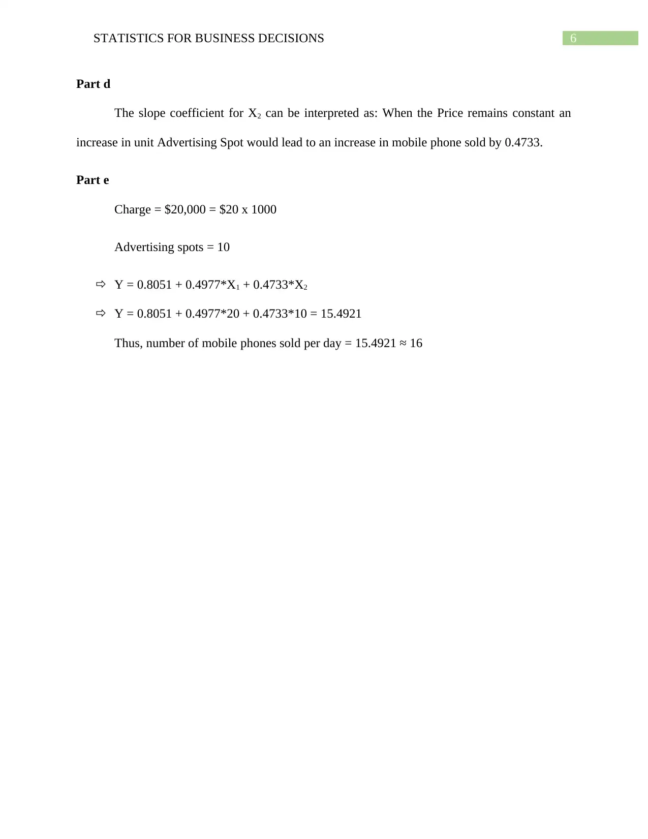
6STATISTICS FOR BUSINESS DECISIONS
Part d
The slope coefficient for X2 can be interpreted as: When the Price remains constant an
increase in unit Advertising Spot would lead to an increase in mobile phone sold by 0.4733.
Part e
Charge = $20,000 = $20 x 1000
Advertising spots = 10
 Y = 0.8051 + 0.4977*X1 + 0.4733*X2
 Y = 0.8051 + 0.4977*20 + 0.4733*10 = 15.4921
Thus, number of mobile phones sold per day = 15.4921 ≈ 16