Statistics for Business: Covariance, Correlation Coefficient, Regression Model, Probability, Mean, Median, Mode, Outliers, Empirical Rule

This document covers topics like Covariance, Correlation Coefficient, Regression Model, Probability, Mean, Median, Mode, Outliers, Empirical Rule in Statistics for Business. It includes a discussion on the relationship between variables, hypothesis testing, probability calculations, measures of central tendency, outliers, and the empirical rule. The document also includes a summary, subject, and references.

STATISTICS FOR BUSINESS
STUDENT ID:
[Pick the date]

Question 1
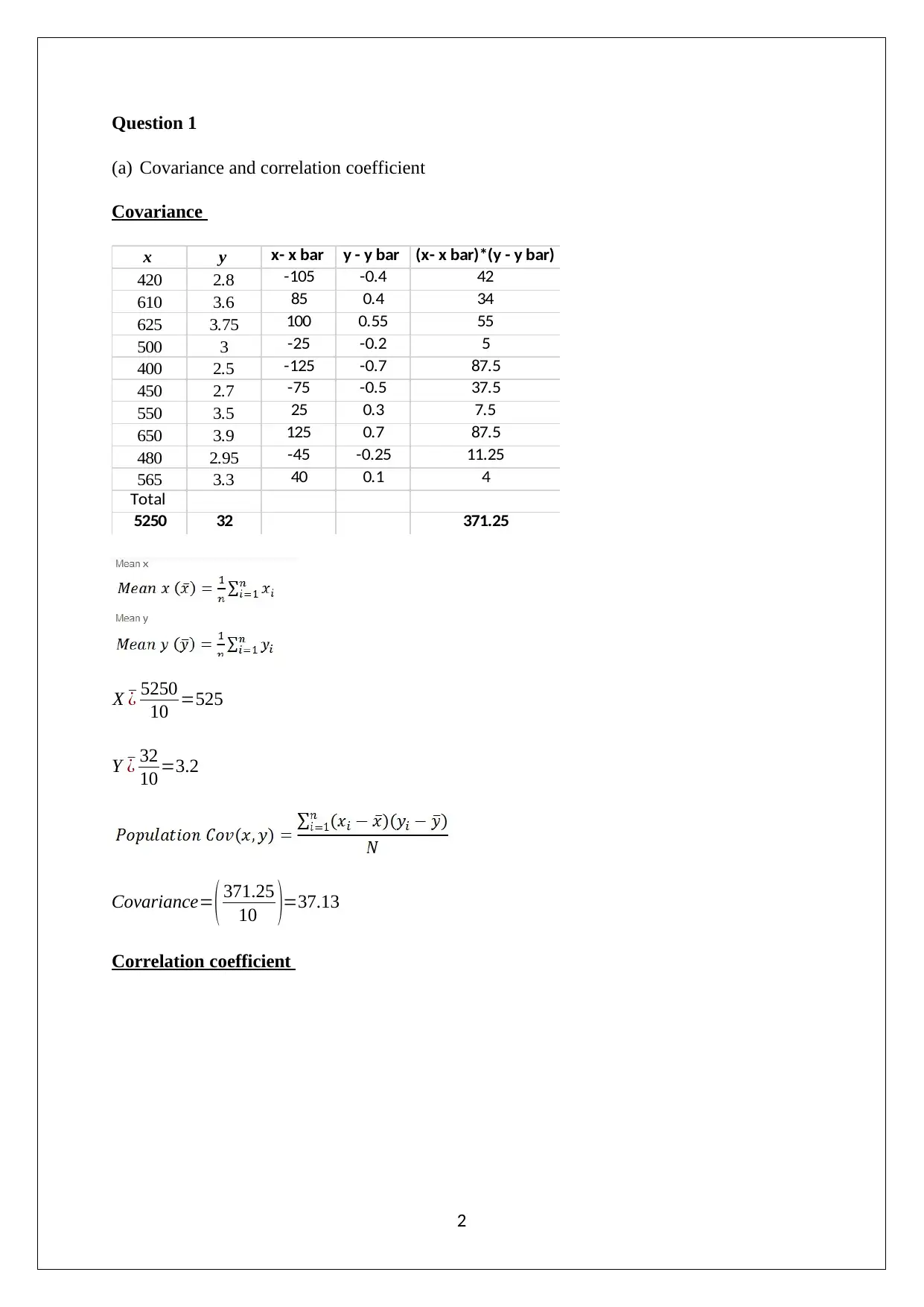
(a) Covariance and correlation coefficient
Covariance
x y x- x bar y - y bar (x- x bar)*(y - y bar)
420 2.8 -105 -0.4 42
610 3.6 85 0.4 34
625 3.75 100 0.55 55
500 3 -25 -0.2 5
400 2.5 -125 -0.7 87.5
450 2.7 -75 -0.5 37.5
550 3.5 25 0.3 7.5
650 3.9 125 0.7 87.5
480 2.95 -45 -0.25 11.25
565 3.3 40 0.1 4
Total
5250 32 371.25
X ¯¿ 5250
10 =525
Y ¯¿ 32
10 =3.2
Covariance= ( 371.25
10 )=37.13
Correlation coefficient
2

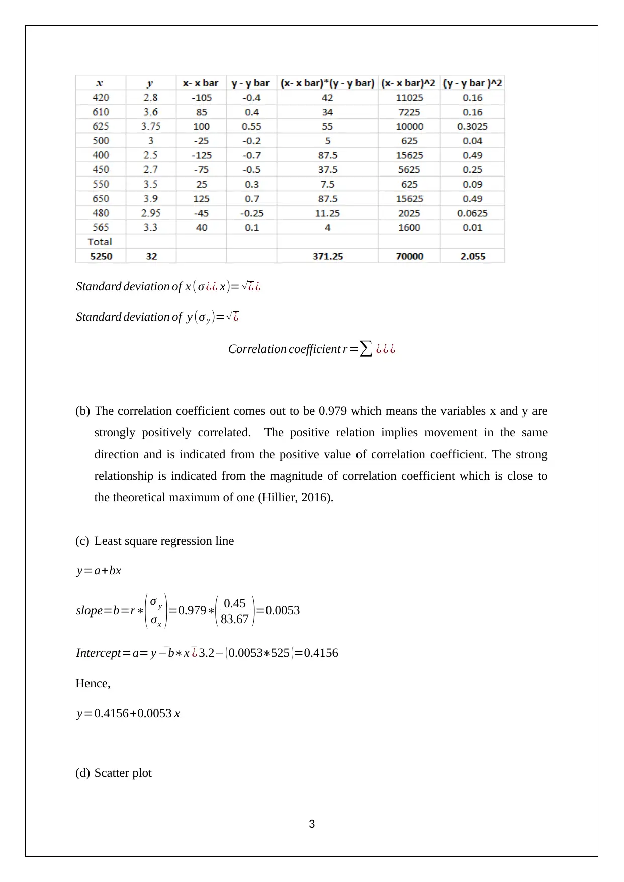
Standard deviation of x ( σ ¿¿ x)= √¿ ¿
Standard deviation of y (σ y )= √¿
Correlation coefficient r =∑ ¿ ¿ ¿
(b) The correlation coefficient comes out to be 0.979 which means the variables x and y are
strongly positively correlated. The positive relation implies movement in the same
direction and is indicated from the positive value of correlation coefficient. The strong
relationship is indicated from the magnitude of correlation coefficient which is close to
the theoretical maximum of one (Hillier, 2016).
(c) Least square regression line
y=a+bx
slope=b=r∗( σ y
σx )=0.979∗( 0.45
83.67 )=0.0053
Intercept=a= y ¯−b∗x ¯¿ 3.2− ( 0.0053∗525 )=0.4156
Hence,
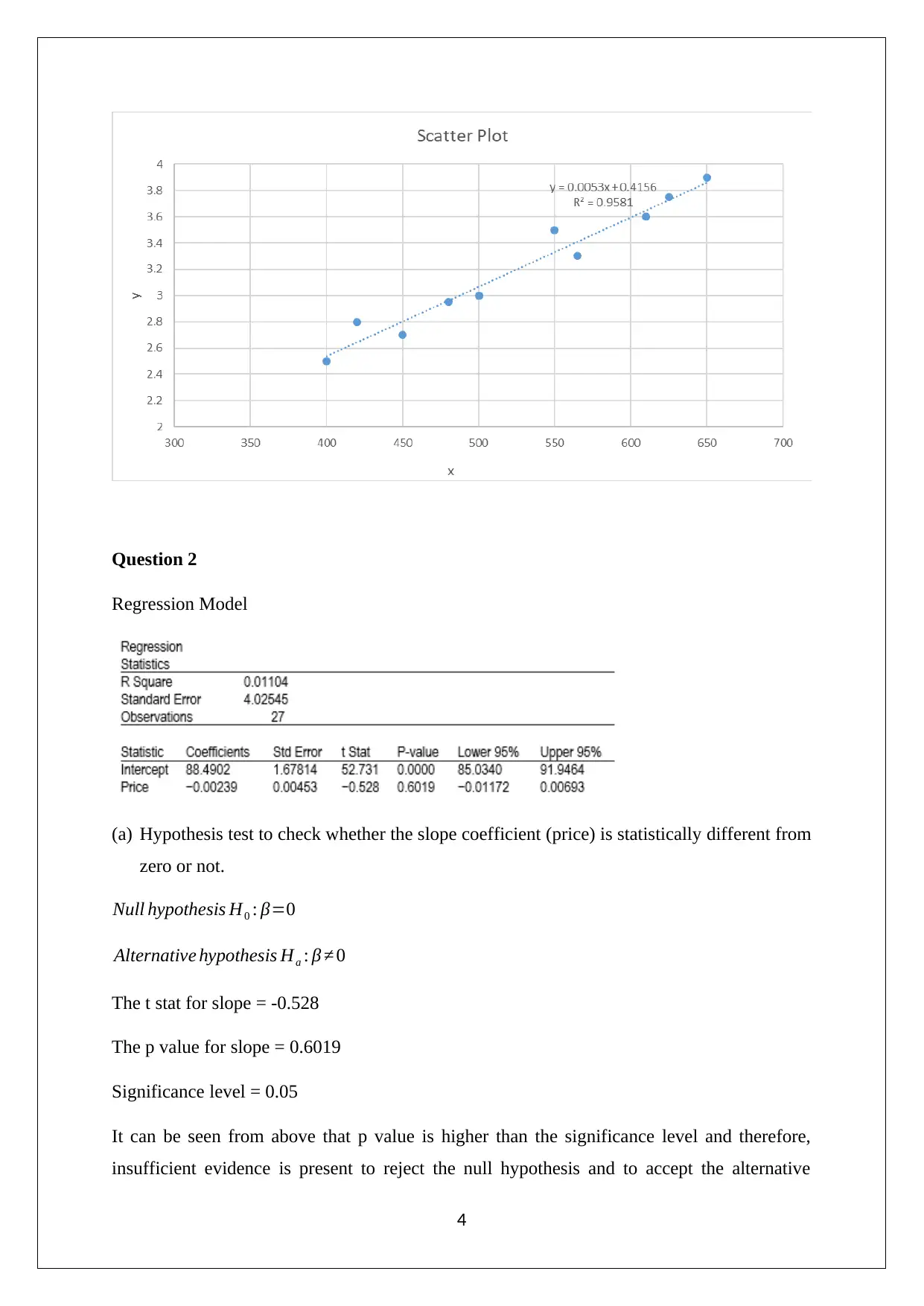
y=0.4156+0.0053 x
(d) Scatter plot
3

Question 2
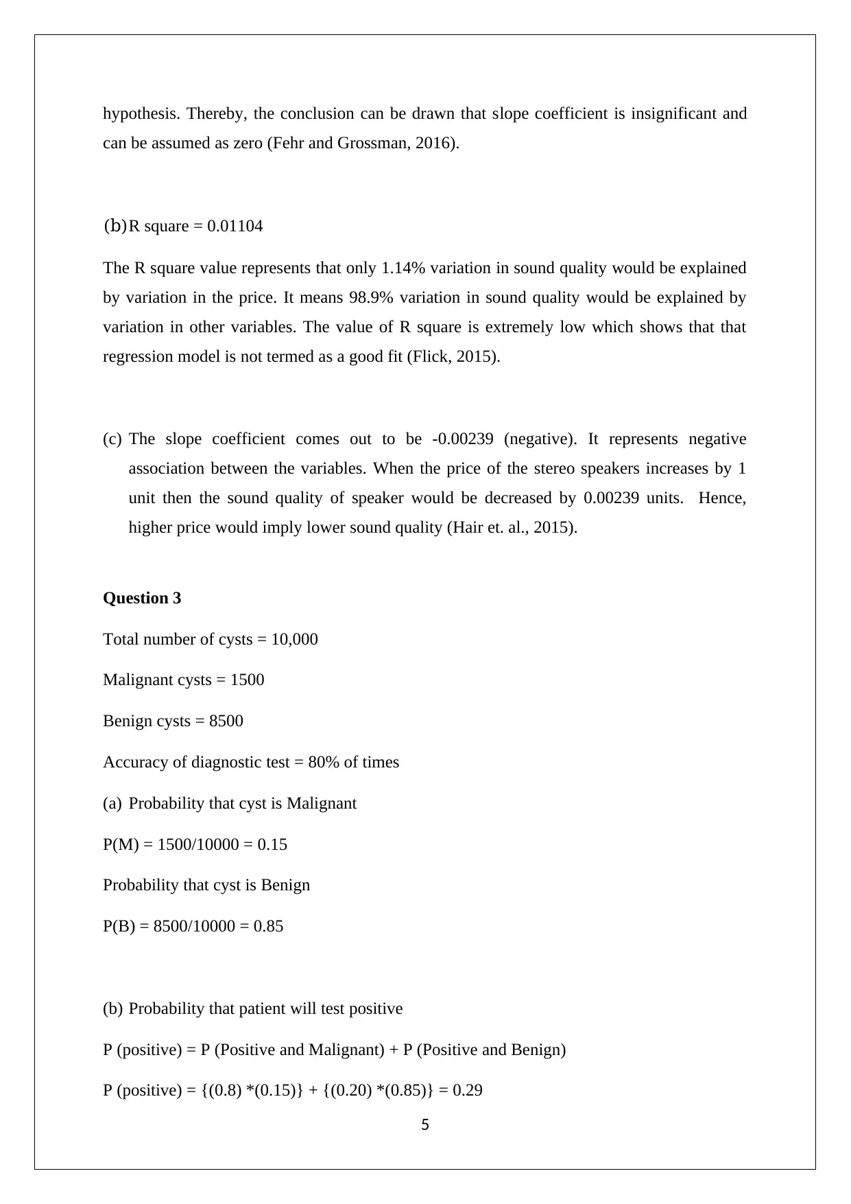
Regression Model
(a) Hypothesis test to check whether the slope coefficient (price) is statistically different from
zero or not.
Null hypothesis H0 : β=0
Alternative hypothesis Ha : β ≠ 0
The t stat for slope = -0.528
The p value for slope = 0.6019
Significance level = 0.05
It can be seen from above that p value is higher than the significance level and therefore,
insufficient evidence is present to reject the null hypothesis and to accept the alternative
4

hypothesis. Thereby, the conclusion can be drawn that slope coefficient is insignificant and
can be assumed as zero (Fehr and Grossman, 2016).
(b)R square = 0.01104
The R square value represents that only 1.14% variation in sound quality would be explained
by variation in the price. It means 98.9% variation in sound quality would be explained by
variation in other variables. The value of R square is extremely low which shows that that
regression model is not termed as a good fit (Flick, 2015).
(c) The slope coefficient comes out to be -0.00239 (negative). It represents negative
association between the variables. When the price of the stereo speakers increases by 1
unit then the sound quality of speaker would be decreased by 0.00239 units. Hence,
higher price would imply lower sound quality (Hair et. al., 2015).
Question 3
Total number of cysts = 10,000
Malignant cysts = 1500
Benign cysts = 8500
Accuracy of diagnostic test = 80% of times
(a) Probability that cyst is Malignant
P(M) = 1500/10000 = 0.15
Probability that cyst is Benign
P(B) = 8500/10000 = 0.85
(b) Probability that patient will test positive
P (positive) = P (Positive and Malignant) + P (Positive and Benign)
P (positive) = {(0.8) *(0.15)} + {(0.20) *(0.85)} = 0.29
5

(c) Probability that patient will test negative
P (negative) = 1 – P (positive) = 1 – 0.29 = 0.71
(d) Probability that patient would has a benign tumour and he/she tests positive
P (Benign / positive) = P (Positive and Benign) / P(Positive) = {(0.20) *(0.85)}/ (0.29) =
0.586
(e) Probability that patient would has a malignant tumour and he/she tests negative
P (Malignant / negative) = P (negative and Malignant) / P(negative) = {(0.20) *(0.15)}/
(0.71) = 0.42
Question 4
(a) Mean. Median and mode
Sorted data in ascending order
6

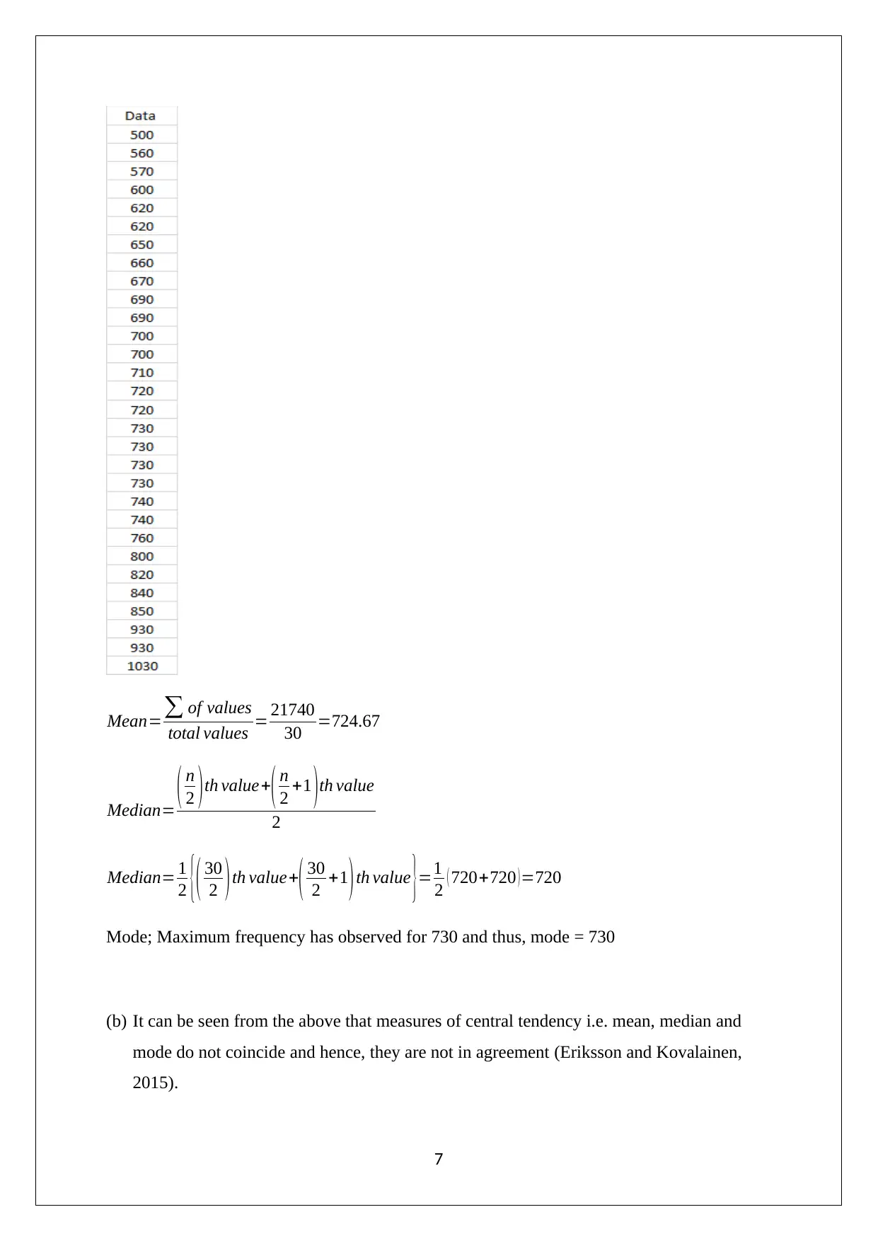
Mean=∑ of values
total values = 21740
30 =724.67
Median= ( n
2 )th value+( n
2 +1 )th value
2
Median= 1
2 {( 30
2 ) th value+( 30
2 +1) th value }=1
2 ( 720+720 ) =720
Mode; Maximum frequency has observed for 730 and thus, mode = 730
(b) It can be seen from the above that measures of central tendency i.e. mean, median and
mode do not coincide and hence, they are not in agreement (Eriksson and Kovalainen,
2015).
7

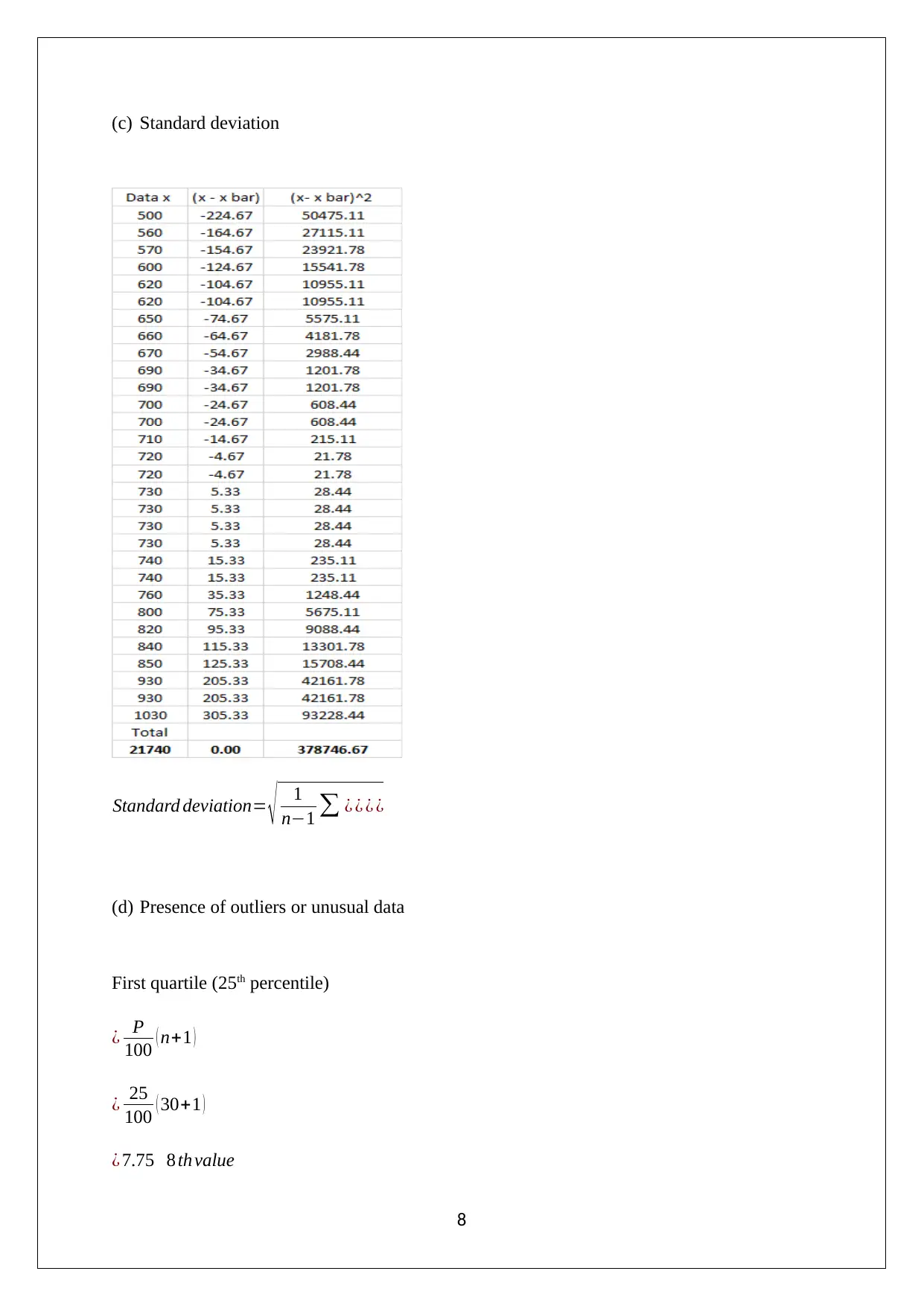
(c) Standard deviation
Standard deviation= √ 1
n−1 ∑ ¿ ¿ ¿ ¿
(d) Presence of outliers or unusual data
First quartile (25th percentile)
¿ P
100 ( n+1 )
¿ 25
100 ( 30+1 )
¿ 7.75 8 th value
8

¿ 660
Now,
Third quartile (75th percentile)
¿ P
100 ( n+1 )
¿ 75
100 ( 30+1 )
¿ 23.25 23 rd value
¿ 760
Inter Quartile Range = Third Quartile – First Quartile
Inter Quartile Range = 760- 660 = 100
Outliers are those which do not lie in the given interval.
Lower limit of interval = First Quartile - 1.5 Inter quartile range
Lower limit of interval = 660 – (1.5*100) = 510
Now,
Upper limit of interval = Third Quartile + 1.5 Inter quartile range
Upper limit of interval = 760+ (1.5*100) = 910
The interval = [510 910)
500, 930, 930 and 1030 are the four values which do not lie in this interval and therefore,
they are termed as outliers.
(e) Empirical rule
It is also known as 8% - 95% - 99.7% rule.
1) 68% rule: It shows that 68%of data values would lie within 1 standard deviation of
mean.
= Mean+/- 1 standard deviation =610.39, 838.95
9

Nearly 70% of data values fall in this interval which means the 68% rule is satisfied.
2) 95% rule: It shows that 95%of data values would lie within 2 standard deviation of
mean.
= Mean+/- 2 standard deviation = 496.10, 953.23
Nearly 96.6% of data values fall in this interval which means the 95% rule is satisfied.
3) 99.5% rule: It shows that 99.5%of data values would lie within 3 standard deviation
of mean.
= Mean+/- 3 standard deviation = 381.82, 1067.51
Nearly 100% of data values fall in this interval which means the 99.5% rule is satisfied.
It can be concluded through Empirical Rule that the data is normally distributed.
10

References
Eriksson, P. and Kovalainen, A. (2015) Quantitative methods in business research. 3rd ed.
London: Sage Publications, pp. 156
Fehr, F. H. and Grossman, G. (2016). An introduction to sets, probability and hypothesis
testing. 3rd ed. Ohio: Heath, pp. 173
Flick, U. (2015) Introducing research methodology: A beginner's guide to doing a research
project. 4th ed. New York: Sage Publications, pp. 199
Hair, J. F., Wolfinbarger, M., Money, A. H., Samouel, P., and Page, M. J. (2015) Essentials
of business research methods. 2nd ed. New York: Routledge, pp. 145
Hillier, F. (2016) Introduction to Operations Research.6th ed.New York: McGraw Hill
Publications, pp. 167
11